Author: Warren Powell

Warren B Powell
Professor Emeritus, Princeton University

I served as Area Editor of Operations Research for eight years (1988-1996) which was a period that taught me a lot about the weaknesses of the standard way of handling papers (send paper to AE who sends it to referees, and then do what the referees say). It took me two years to realize that this approach just wasn’t working.  I came up with an entirely new approach which I summarized in a memo available here.  This web page is a brief summary of the core ideas. 

It all begins with three principles:

• Let authors be authors
• Let editors be editors
• Let referees be referees

I explain below.

Let authors be authors

The responsibility of authors is to write, as clearly as possible, a paper that offers something new.  For this reason, the author is in the best position to tell us what is new and significant in their paper.

An idea I was given by Mark Daskin (who adopted it from his colleague Phil Jones) is to include, typically in the next-to-last paragraph of the introductory section, a paragraph that begins with “This paper makes the following contributions.”  The rest of this paragraph should be a list that contains what the author feels are publishable contributions.  The last paragraph should give the organization of the paper.

Note that a contribution is not a list of what the paper has done.  Implicit in each contribution is an implicit claim that it is original and significant.  In other words, each contribution should contain a claim that may be verified by knowledgeable reviewers. 

Let editors be editors

First let me emphasize: there is more to editorial work than just picking an AE or reviewers, sending it out, and then repeating whatever the referees tell you to do.  When I was active in editorial work, we called these people “mailboxes.”  

Given the list of contributions, the first responsibility of any editor is to read the list and then make a judgment of the form “If this claimed contribution is true, does this seem to be of sufficient interest for the readers of my journal.”  

My experience with this process quickly revealed that most authors do not know how to write a list of contributions.  The key feature of any contribution is that it should have a claim that can be verified by a knowledgeable reviewer.  When the contributions did not meet this standard, I would return the paper and request a revision (sometimes I would just ask for a revision in email, that I would then forward to the AE).  Often it would take two or three iterations for me to get a list of contributions that I felt I could then send through the review process.

Once I felt I had a valid list of contributions, I would make an initial assessment of whether the paper appeared to be publishable if all (or at least some of) the claims were true.  I expected the AE to also look at the list of contributions and make the same assessment.  The paper would then go to reviewers, with a request that part of their report would focus specifically on whether the claimed contributions were original and significant (that is, of publishable interest).  

Finally, when the reviews are returned, the editors should first look at the reviewers’ assessment of the claimed contributions.  

Side note: I include the “statement of contribution” paragraph in every one of my papers.  Simply stunning how often the editors just ignore it.

Let referees be referees

With surprising frequency, referees would appoint themselves as authors, and they would decide how they think the paper should be written.  

While referees should read the entire paper and feel free to make any comments that they feel would improve the paper, most important should be their assessment of the list of claimed contributions.  Even if some contributions are not deemed original or significant, the reviewer may confirm one or more contributions that an editor feels are enough to justify publication.  This assessment is key, and should be kept separate from other statements that a reviewer may make.

I often found reports that intermingled minor edits, fixable problems, and fundamental issues that are not fixable within the scope of the paper (a revision would really be a new paper).  

Closing thoughts

This approach to reviewing puts the responsibility on authors to identify what is most important about their paper.  This simplifies the review process by focusing the attention of editors and referees on what the author feels is most important.  This should also help separate the fundamental decision of whether to accept a paper (including some form of revision) versus an outright rejection.

This approach reduces the tremendous amount of noise that currently exists in the review process.  It helps reviewers organize their comments in a way that is most helpful to the editors, which is to separate the topics that are most relevant to accept or reject decisions, versus recommendations to authors that are primarily designed to improve the paper.

 

 

Warren B. Powell
Professor Emeritus, Princeton University

My book, Reinforcement Learning and Stochastic Optimization, synthesizes 15 different fields that work on sequential decision problems,  but there is a price: it is an 1100 page book.  xxxxxxxT

This webpage is designed to guide newcomers to the field that I have been calling sequential decision analytics. It will start with video tutorials, then transition to a book I wrote for my undergraduate course, and then I will start stepping into the “big book” which can be done in stages.

Step 1: Video tutorials

• I recommend starting with the short (40 minute) video introduction:

https://tinyurl.com/sdafieldyoutube/

• I then suggest the four-part tutorial (approximate 100 minutes total) which expands the tutorial above with more examples, a more complete discussion of modeling, and a more complete discussion of all four classes of policies.

• https://tinyurl.com/SDAPartI
• https://tinyurl.com/SDAPartII
• https://tinyurl.com/SDAPartIII
• https://tinyurl.com/SDAPartIV

Step 2: The “beginner” book

I wrote this book for an undergraduate course, but it is ideal for almost anyone who wants to first understand how to think about sequential decision problems.  An introduction to the book is available at

Sequential decision analytics and modeling

The book can be downloaded by clicking here. 

This book uses a teach by example style.  Chapter 1 gives an introduction to the universal modeling framework.  Then, all the remaining chapters (with the exception of chapter 7) are examples, each written using the same outline, and each chosen to bring out different modeling issues.  Chapter 7 pauses to illustrate the key ideas using the examples in the first six chapters.  This book is very easy to skim.

Step 3: Reading the “big book”

At this point, you need a copy of Reinforcement Learning and Stochastic Optimization (RLSO). The print version can be purchased on Amazon, but do not by the kindle version if you are interested in an electronic version.  Instead, get the Wiley e-book version from here – they have done an exceptional job.

Once you have the book, I suggest:

• Read/skim chapter 1, which provides an overview of the book (this will overlap somewhat chapter 1 of SDAM).
• Pay special attention to “Section 1.8 – How to read this book”.  This section outlines the organization of the book, and notes that sections marked by an * can be skipped the first time through the book.  This will dramatically shorten the book on a first read.  
• Also note that chapter 11 provides an overview of all four classes of policies, and provides guidance on how to choose among the policies.  If you have a specific problem you are trying to solve, this may help you avoid going through chapters 12-19 which cover:
  • Chapter 12 – Policy function approximations (PFAs)
  • Chapter 13 – Cost function approximations (CFAs)
  • Chapters 14-18 – Policies based on value function approximations (VFAs) – This is the material most often identified with “reinforcement learning” or “approximate dynamic programming”
  • Chapter 19 – Direct lookahead approximations (DLAs) – This chapter presents two important subclasses of policies:
    • Deterministic lookahead models (possibly parameterized)
    • Stochastic lookahead models – Here I review how to design policies within the lookahead model.

Step 4: Self-study

Finally, I have a series of suggested ways of teaching this material at

https://tinyurl.com/RLSOcourses/

At the top I have designed a “Weekly seminar series” where I have outlined the material that a group of students or professionals could work through the material in the book.  These topics can also be used as guidance for individual self study.

Also – I make available three important chapters from the book webpage (https://tinyurl.com/RLandSO/) where you can download chapter 1 for an overview (also chapters 9, on modeling, and 11, on the four classes of policies).

Step 5: Other educational material

I maintain a webpage of resources for the field of sequential decision analytics at:

https://tinyurl.com/sdalinks/ (or https://castle.princeton.edu/sdalinks)

 

Warren B Powell

After a post on modeling sequential decision problems (aka RL problems), I was asked: “Are you using “x” for control/decision here? For RL or DP it is more common to use x/s for state, u for control, and r/c for reward/cost. Furthermore, what do these W variables mean?”

For many years, the RL community followed the notation of discrete Markov decision processes dating back to Bellman where “s” was state, “a” was a discrete action, p(s’|s,a) was the one-step transition matrix and r(s,a) was the single period reward.  This is the notation used throughout Sutton and Barto’s books.

But today, Dimitri Bertsekas’ books have received considerable attention in the RL literature.  Dimitri uses classical notation from optimal control where x is the state, u is the control, and the state evolves according to the one-step transition function written using

x_{k+1} = f(x_k,u_k,w_k)                                                                            (1)

where w_k is a “noise” term that is random at “time” k.

This is a mess, and it is time to fix this.

We have two books that have received considerable attention in the RL community (by Sutton and Barto’s Reinforcement Learning: An introduction and Bertsekas’ Dynamic Programming and Optimal Control: Approximate Dynamic Programming (4th edition), with completely conflicting notational systems, both of which have serious problems.  Below I discuss how I have solved these problems in my new book, Reinforcement Learning and Stochastic Optimization: A unified framework for sequential decisions.

State variables:

“s” (in some form) is widely used as a state variable in dynamic programming which has been adopted throughout the CS/RL community.  By contrast, “x” is the standard notation in the controls community.  Not only is “s” (or S_t or S^n) a natural and widely used choice, next we are going to make the argument that “x” has a major conflict and should be avoided.

There are many problems where the natural index is a counter (number of observations, arrivals, experiments, iterations, …).  In that case, I use S^n, x^n and W^{n+1}.  I put this in the superscript since there are problems where you have time (such as hour of week) as well as iterations (the nth week), so you might write S^n_t or x^n_t.  See my discussion of notation in section 9.2 of RLSO.

There is considerable confusion in the interpretation of state variables.  The books on MDP/RL never define a state variable, while there are many books in the optimal control literature that provide explicit definitions.  Click here for a more in-depth discussion of this rich topic.

Decision variables:

“x” has been used by the math programming community since the 1950s, and is standard notation around the world.  While “a” is standard notation for dynamic programming, in the vast majority of applications it is discrete.  By contrast, “x” may be binary, discrete, continuous scalar, as well as continuous or discrete vectors (in other words, anything).  “x” was also adopted by the bandit community in computer science (which is closely associated with reinforcement learning), which means we have two communities, both in computer science and both associated with reinforcement learning, using two different notations for decision. 

In my view, “x” is easily the most obvious choice for decision, which gives us a notational system that is welcoming to the field of math programming.  This said, I do not feel there is any problem continuing to use “a” for discrete actions; not only is there a long history behind this notation (and I think this is important to respect), the idea of seeing “a” and then knowing that we are dealing with discrete actions has a certain appeal.  If engineers still want to use “u” for continuous controls, I have no objection, but I encourage people new to the field to adopt “s” (or “S“) for state.

I have seen people object to x as a decision variable given its widespread use in machine learning.  I do not feel there is a conflict here, since there are many problems where the input data to a machine learning problem is a decision (see, for example, the multiarmed bandit community).  There are, of course, many settings in machine learning where we cannot control what we observe, just as there are settings where there is a mixture (I cannot control the attributes of a patient, but I can control what drug I prescribe, and the combination of attributes and drug influence how the patient responds).  

Exogenous information

Fully sequential decision problems (decision, information, decision, information, ….) have to capture an exogenous information process that represent new information arriving to the system after a decision has been made.

In the MDP/RL modeling framework, this information is buried in the one-step transition matrix, which hides both the modeling of the exogenous information process (which is an important dimension of many problems) as well as how the system evolves over time. 

The optimal control community has long used the notation

x_{k+1} = f(x_k,u_k,w_k). 

The reason why the “noise” variable w_k is random at “time” k is a holdover from continuous time models where w_t is the noise over the interval [t, t+dt].  But when we make the transition to discrete time, it makes more sense to require that any variable indexed by t be known at time t (“F_t-measurable”).  I use capital W_{t+1} (probabilists like capital letters for their random variables) for the exogenous information (my term) that arrives after we make a decision.

The transition function

The RL/MDP community likes to model transitions as a transition matrix p(s’|s,a) (“transition kernel” if s is continuous), but this is virtually never computable.  Even if you try to compute it, you have to start with the one-step transition function.  It makes much more sense to use the one-step transition function from control theory.  I don’t like using [f(...) since this piece of notation is too useful for other purposes, so, using our new notation for exogenous information, state evolutions are written using

S_{t+1} = S^M(S_t,x_t,W_{t+1}),

where S^M(...) is the “state transition model” (or just “model”).

I have heard experts in RL tell me that they just “simulate the transition matrix.”  No-one would ever compute a one-step transition matrix and then use it to draw samples of a transition (although this is possible).  Any implementation of an RL algorithm uses a transition function rather than a transition matrix (or kernel).  

Once you have the transition function and a model of the exogenous information process W_t, you can in principle find the one-step transition matrix (or kernel), but only in principle – almost never in practice.

Objective function

The canonical model of a dynamic program in the MDL/RL community will list the reward r(s,a) as one of the four modeling elements.  This is the one-step reward (I like to use C(S_t,x_t) for the which depends on the information in the state variable S_t and the decision x_t.  This is the single-step reward/contribution/cost function, but it is not the objective function!

The most common way to write an objective fun for dynamic programs (this is a specific version that I call the cumulative reward):

\max_\pi \mathbb{E} \left\{\sum_{t=0}^T C(S_t,X^\pi(S_t))|S_0\right\}.

The objective is to find the best policy (at least, aspire to).  This goal is completely missing from the standard MDP/RL model.  Note that there are problems (in particular arising in offline settings such as laboratory experiments or simulators) where we might write our objective as

\max_\pi \mathbb{E} \left\{F(x^{\pi,N},W)|S_0\right\}.

We would use this objective if we were optimizing the parameters of a simulator (see Chapter 7 of RLSO for a discussion of cumulative and final reward objectives, or Chapter 9, section 9.8 of RLSO for a more thorough discussion of objectives).  We might even use a risk metric.  Whatever choice we make, it has to be specified in our model!  

Final remarks

My notation builds on the most important modeling styles from the Markov decision process, optimal control, math programming, machine learning and simulation communities.  I think it is important for students new to the problem class to recognize that the study of sequential decision problems needs to stand on the shoulders of all of these fields.  My new book RLSO is built on this notational framework.

 

 

 

September 1, 2020

Professor of Operations Research and Financial Engineering Warren Buckler Powell will transfer to emeritus status on September 1, 2020, after 39 years on the faculty.

Warren graduated from Princeton University in 1977 with a bachelor’s degree in civil engineering specializing in transportation systems, and then received his Ph.D. from MIT, also in transportation systems. While at MIT he was introduced to the field of operations research which he describes as the “mathematics of everyday life” and realized that he had found his calling. He returned as a faculty member in civil engineering at Princeton in 1981, accepting the challenge of starting an operations research program, where he saw the opportunity to bring the mathematical foundations directly to engineers solving real problems. He helped to transition an existing program in “Basic Engineering” to “Engineering and Management Systems,” and moved the existing transportation program to the new EMS program doing operations research.

Warren’s career coincided with the deregulation of freight transportation in 1980, creating a sudden market for advanced planning tools at a time when computers were just starting to become useful. He was quickly attracted to the analytical challenges faced by the trucking industry. In the 1980s, he developed the first interactive optimization model for less-than-truckload (LTL) carriers, which operated hub and spoke networks similar to airlines (this model was written in Fortran, on an IBM mainframe). During the 1980s, 80 percent of LTL carriers went out of business. By the 1990s, virtually the entire industry was using the model he developed (“SuperSPIN”), which stabilized the entire industry. SuperSPIN was used to plan Roadway Package Express (now known as FedEx Ground) and American Freightways (now known as FedEx Freight). He also enjoyed 25 years of funding from what is now known as YRC, currently the second largest less-than-truckload motor carriers, for which he developed strategic and operational planning models that are still in use today.

His passion, however, was the industry known as truckload trucking, which can be thought of as Uber for freight: the problem is to decide which driver should move each load of freight, where the choice of drivers and loads had to reflect conditions after the load was delivered, which might be up to three or four days into the future. The problem combined high-dimensionality, requiring the matching of hundreds to thousands of drivers and loads at the same time, while also handling the uncertainty of the future. This was his first introduction to stochastic optimization.

Modeling and designing computationally tractable algorithms for this problem proved to be Warren’s defining problem, and it started his tour through what he would later call the “jungle of stochastic optimization,” which addresses the broad problem of making decisions over time under uncertainty. He would later identify over 15 distinct academic communities that all contributed to mathematical models and algorithms for sequential decision problems in the presence of uncertainty, but not one provided the tools to solve his fleet management problem.

In 1990, he founded CASTLE Lab, which was originally an acronym for Computational Stochastic Transportation and Logistics Engineering, but later was adjusted to the more modern ComputAtional STochastic optimization and LEarning. In the 1990s, CASTLE Lab became renowned for bringing advanced analytics to a wide range of problems in transportation and logistics, spanning LTL and TL trucking, locomotive management for rail, military airlift, drayage, spare parts management, vehicle routing and scheduling, and supply chain management.

Most prominent was Warren’s development of a class of techniques in an emerging field known as “approximate dynamic programming” (ADP), which had been limited to simple “mouse-in-a-maze” problems or engineering control applications. Warren was the first to develop ADP methods for high-dimensional control problems (his “decisions” had over 50,000 dimensions) using a modeling device called the “post-decision state.” This work would lead to his popular book, Approximate Dynamic Programming: Solving the Curses of Dimensionality.

In the early 2000s, he took advantage of the downturn from the dot-com era to transition to new problems, settling initially on energy systems. He founded PENSA (Princeton Laboratory for Energy Systems Analysis) and brought the same research model to energy problems to help address the emerging problems related to handling the variability and uncertainty of increasing investments in wind and solar. In fact, it was his work in freight transportation that combined optimization and uncertainty that launched his first project with Lawrence Livermore to optimize an energy storage system.

By 2015, he had brought in over $7.5 million in funding from the Department of Energy, Lawrence Livermore, NRG Energy, and a large grant from SAP to support energy systems research. This work produced the first detailed model of PJM Interconnections, the grid operator for the mid-Atlantic states serving 60 million people. His other work spanned bidding and forecasting, but also produced what is today the most comprehensive set of models and algorithms for energy storage, a critical technology for handling the variability and uncertainty of wind and solar.

During this period, Warren continued to mature in his formal methodological research in stochastic optimization, which emerged with his work on approximate dynamic programming. An important issue that arises throughout the design of ADP algorithms is known as the “exploration vs. exploitation” problem: do we make a decision because it appears best (based on current estimates), or to help refine our estimate of the value of the state the decision takes us to?

He decided to tackle the “exploration vs. exploitation” problem as an area of research, which produced his book Optimal Learning, and a series of papers developing a powerful learning policy that he called the “knowledge gradient.” He realized the broad appeal of this idea and introduced a popular undergraduate elective course called “Optimal Learning.” Undergraduates have been attracted by the broad applicability of the core problem of optimal learning and the relative simplicity of the tools.

Warren’s work in optimal learning led to a major grant with the Air Force focusing on sequential design of experiments for materials science, which brought him into an entirely new community with a new set of questions. This work required interactions with materials scientists, electrical engineers, and chemical engineers, and produced new tools that apply to anyone working in the laboratory sciences.

By 2010, Warren had been exposed to an exceptionally wide range of sequential decision problems. This experience led to a series of articles, starting in 2014 with a tutorial called “Clearing the Jungle of Stochastic Optimization,” progressing through two articles in 2016 and 2019 that developed a unified framework for stochastic optimization that bridges all 15 communities that work on sequential decision problems. In 2018-19, he put together two new courses, one graduate and one undergraduate, that brought these ideas (traditionally limited to mathematically sophisticated communities) to a broad audience. He wrote an online book for the undergraduate course that uses a teach-by-example style, and is nearing completion of a graduate-level book, all available at jungle.princeton.edu.

Warren’s work was supported by over $50 million in funding from over 70 different projects, including almost 40 projects from a range of industrial companies, and over 30 government grants from the National Science Foundation, the Air Force Office of Scientific Research, and the Department of Energy.

Warren’s research produced 250 publications, most in top-tier journals that have attracted over 18,000 citations. He has written two books, Approximate Dynamic Programming (now in its second edition) and Optimal Learning, along with an online book: Sequential Decision Analytics and Modeling. As he retires, he is nearing completion of Reinforcement Learning and Stochastic Optimization: A Unified Framework for Sequential Decisions.

Warren is perhaps most proud of his 60 graduate students and post-docs. He retires with almost 30 placements in academia (including Cornell University, Columbia University, University of Pennsylvania, London School of Economics, Lehigh University, Stevens Institute of Technology, University of Toronto, and Hong Kong University of Science and Technology) and research labs (Lawrence Livermore, IBM TJ Watson, AT&T Bell Labs). He also supervised over 200 senior theses and independent projects.

Over his career, his work contributed to three startups. The first, Princeton Transportation Consulting Group, was started in 1988. PTCG brought his software for both less-than-truckload and truckload trucking to rapidly evolving post-deregulation market. In 1995 he started Transport Dynamics. His third company, Optimal Dynamics, was started in 2016 with his son Daniel Powell as president and CEO, and Warren is looking to continue working with Optimal Dynamics after he retires from Princeton.

Warren is looking forward to bringing his new ideas for sequential decision analytics to an international audience, starting with a series of tutorial workshops (all the material is available at jungle.princeton.edu). He is also looking forward to developing his first MOOC course, and has been actively interacting with researchers around the world. While he will miss teaching at Princeton, he is looking forward to bringing these ideas to a much larger audience.

Warren B. Powell

Everyone wants the simplest possible algorithms,  especially in machine learning and reinforcement learning/stochastic optimization.  Some examples are:

• Stepsize rules for stochastic gradient algorithms (virtually all have at least one tunable parameter).
• Order-up-to policies for inventory problems.
• Control limit policies:
  • Vaccinate people older than \theta.
  • Put on a coat when it is colder than \theta degrees).
  • Purchase the product if the price is less than \theta.
• Parameterized optimization models (see parametric cost function approximations).
• Most algorithms for derivative-free stochastic optimization.
• Upper confidence bounding policies for bandit problems, such as:

X^\pi(S^n|\theta)=argmax_x({\bar \mu}^n_x + \theta {\bar \sigma}^n_x)                                          (1)

There are endless examples of methods for making decisions which involve tunable parameters.  But as I repeat several times in my book, “the price of simplicity is tunable parameters… and tuning is hard!”

This webpage highlights some important issues in the design of algorithms that have been largely overlooked in the research literature dealing with learning/stochastic optimization.  

Tuning as an optimization problem

Tuning can be stated as an optimization problem typically using one of two optimization formulations.  The most classical form is given by

max_\theta F(\theta) = \mathbb{E}\{F(\theta,W)|S^0\}                                                                (2)

If we are tuning the parameters of a policy (such as equation (1)) that has to be evaluated over time, we might write

max_\theta \mathbb{E}\left\{\sum_{t=0}^TC(S_t,X^\pi(S_t|\theta))|S_0\right\}                                                    (3)

where S_{t+1}=S^M(S_t,X^\pi(S_t|\theta),W_{t+1}) and where the sequence of random variables W_1, \ldots, W_T might come from a mathematical model (using Monte Carlo simulation) or from history.

The optimization problems in (2) and (3) can be approached using either derivative-based (see chapter 5 in RLSO) or derivative-free (see chapter 7 in RLSO) stochastic search problems.  Both of these chapters make the point that any stochastic search algorithm can be posed as a sequential decision problem (which has its own tunable parameters).

The importance of tuning

Experimentalists are generally aware of the importance of tuning, but the need to tune and re-tune parameters is easy to overlook, often because it is time consuming, and has to be done manually.  The figure below on the left shows the results of parameter tuning when starting the process in one of four ranges (indicated by the four colors).  The fourth range (farthest to the right) shows the stochastic optimization algorithm producing poor solutions.  The figure on the right shows consistently better performance for all four starting regions, but this was achieved only by re-tuning the stepsize rule used by the stochastic gradient algorithm.

Tuning the parameters in the stepsize rule is easy to overlook.  Good experimentalists recognize the need to tune these parameters, but the idea of re-tuning when we change the starting point (for example) is not at all standard practice, and may explain why algorithms can fail.

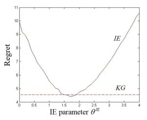
The figure to the right shows the regret (smaller is better) comparing the UCB policy (known as interval estimation) in equation (1) above, to a more sophisticated policy called the knowledge gradient (see section 7.7.2 in RLSO) which is a one-step lookahead. KG does not have any tunable parameters, but requires some moderately sophisticated calculations.  The figure demonstrates that the much simpler UCB policy (interval estimation) can outperform KG, but only if the tunable parameter \theta is carefully tuned.  

Tuning can be quite difficult.  Typically we would perform tuning with a simulator, as was done in the figure above for tuning \theta in the UCB policy in equation (1).  However, the simulations are extremely noisy.  To obtain the smooth curve in the figure above, we had to run 1000 simulations for each value of \theta.  The optimal value also depends on the learning budget.  The best value of \theta would change if we have a budget of 50 experiments or 500, as well as being dependent on other problem parameters.

Dependence on the initial state

The optimization problem in equation (2) expresses the dependence of the problem on the initial state S^0, where we assume we have a search algorithm that produces the sequence 

S^0,\theta^0,W^1,S^1,\theta^1,W^2, \ldots, S^n,\theta^n,W^{n+1}, \ldots, S^N,\theta^N.

In the objective function in (3), we assume we have a temporal process that can be written

S_0,x_0,W_1,S_1,x_1,W_2, \ldots, S_t,x_t,W_{t+1}, \ldots, S_T,x_T.

where x_t = X^\pi(S_t|\theta).  We then have an outer loop that searches for \theta using equation (2) where 

F(\theta,W) = \mathbb{E}\left\{\sum_{t=0}^TC(S_t,X^\pi(S_t|\theta))|S_0\right\},

starting with S_0 = S^0.  

So, regardless of whether we are using the objective function (2) or (3), we start with an initial state S^0.  Now let \theta^{\pi,N} be the value of \theta after we have run N iterations of an “algorithm” (search policy) \pi.  We might write \theta^{\pi,N} as \theta^{*} to indicate that it is in some sense “optimal,” but what this ignores is that the solution \theta^{\pi,N} depends on S^0, which means we really would like to have the function \theta^{\pi,N}(S^0).  Of course, no-one ever tries to derive this function, which means that we face the need to re-tune \theta^{\pi,N} any time S^0 changes.

So just what is in S^0?  It really covers anything that affects the behavior of the underlying function F(\theta) or the algorithm that searches for \theta^{\pi,N} (including the initial value \theta^{0}).

The dependence on S^0 has been largely overlooked in the algorithmic literature.  In fact, writing the dependence of the objectives on S^0 (as is done in (2) and (3)), is not standard in the stochastic optimization literature (note that it is standard in my book RLSO, for precisely this reason).  

Types of tunable parameters

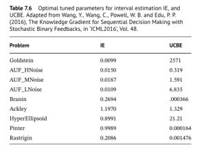
The point needs to be made that not all tunable parameters are made equal.  The issue really boils down to scaling.  The table to the right shows how two different policies for making decisions: The one under “IE” is given by equation (1)), while the one under “UCBE” uses a different term for capturing uncertainty.  The table shows much more variation for the UCBE policy than the IE policy.

In a nutshell, the more work that goes into designing a function, the less tuning that will be required.  A powerful strategy for making sequential decisions is called the “cost function approximation” (see here for a description). CFA policies start by formulating a decision problem as a deterministic optimization model, and then introduces parameters that are designed to make it work better over time, under uncertainty.  The initial deterministic optimization problem captures a lot of structure which minimizes scaling as an issue.

Recommendations

Tuning has not received the attention it deserves in the algorithmic research literature.  For example, there is an extensive literature for searching over a discrete set of alternatives to learn the best (equation (1) is one example).  There are many hundreds of papers proving various regret bounds on these policies, without even mentioning that \theta has to be tuned, which in turn means there is no discussion of how it should be tuned.  And as we see in the previous figure, tuning matters.

I believe that every algorithmic paper should be accompanied by a discussion of the requirements for parameter tuning.  The discussion should comment on scaling, the level of noise when running simulations, and objective functions for both offline tuning using a simulator (equation (2)) or online tuning in the field (equation (3)).  Experimental testing of an algorithm should include experiments from the tuning process.