Warren B. Powell
Everyone wants the simplest possible algorithms, especially in machine learning and reinforcement learning/stochastic optimization. Some examples are:
- Stepsize rules for stochastic gradient algorithms (virtually all have at least one tunable parameter).
- Order-up-to policies for inventory problems.
- Control limit policies:
- Vaccinate people older than
.
- Put on a coat when it is colder than
- Purchase the product if the price is less than
- Vaccinate people older than
- Parameterized optimization models (see parametric cost function approximations).
- Most algorithms for derivative-free stochastic optimization.
- Upper confidence bounding policies for bandit problems, such as:

There are endless examples of methods for making decisions which involve tunable parameters. But as I repeat several times in my book, “the price of simplicity is tunable parameters… and tuning is hard!”
This webpage highlights some important issues in the design of algorithms that have been largely overlooked in the research literature dealing with learning/stochastic optimization.
Tuning as an optimization problem
Tuning can be stated as an optimization problem typically using one of two optimization formulations. The most classical form is given by

If we are tuning the parameters of a policy (such as equation (1)) that has to be evaluated over time, we might write

where 

The optimization problems in (2) and (3) can be approached using either derivative-based (see chapter 5 in RLSO) or derivative-free (see chapter 7 in RLSO) stochastic search problems. Both of these chapters make the point that any stochastic search algorithm can be posed as a sequential decision problem (which has its own tunable parameters).
The importance of tuning
Experimentalists are generally aware of the importance of tuning, but the need to tune and re-tune parameters is easy to overlook, often because it is time consuming, and has to be done manually. The figure below on the left shows the results of parameter tuning when starting the process in one of four ranges (indicated by the four colors). The fourth range (farthest to the right) shows the stochastic optimization algorithm producing poor solutions. The figure on the right shows consistently better performance for all four starting regions, but this was achieved only by re-tuning the stepsize rule used by the stochastic gradient algorithm.
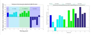
Tuning the parameters in the stepsize rule is easy to overlook. Good experimentalists recognize the need to tune these parameters, but the idea of re-tuning when we change the starting point (for example) is not at all standard practice, and may explain why algorithms can fail.
The figure to the right shows the regret (smaller is better) comparing the UCB policy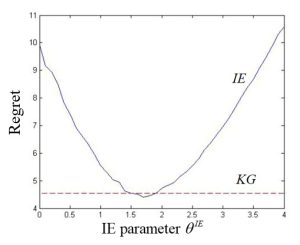 (known as interval estimation) in equation (1) above, to a more sophisticated policy called the knowledge gradient (see section 7.7.2 in RLSO) which is a one-step lookahead. KG does not have any tunable parameters, but requires some moderately sophisticated calculations. The figure demonstrates that the much simpler UCB policy (interval estimation) can outperform KG, but only if the tunable parameter
Tuning can be quite difficult. Typically we would perform tuning with a simulator, as was done in the figure above for tuning
Dependence on the initial state
The optimization problem in equation (2) expresses the dependence of the problem on the initial state 

In the objective function in (3), we assume we have a temporal process that can be written

where 

starting with 
So, regardless of whether we are using the objective function (2) or (3), we start with an initial state 


So just what is in 

The dependence on
Types of tunable parameters
The point needs to be made that not all tunable parameters are made equal. The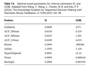 issue really boils down to scaling. The table to the right shows how two different policies for making decisions: The one under “IE” is given by equation (1)), while the one under “UCBE” uses a different term for capturing uncertainty. The table shows much more variation for the UCBE policy than the IE policy.
In a nutshell, the more work that goes into designing a function, the less tuning that will be required. A powerful strategy for making sequential decisions is called the “cost function approximation” (see here for a description). CFA policies start by formulating a decision problem as a deterministic optimization model, and then introduces parameters that are designed to make it work better over time, under uncertainty. The initial deterministic optimization problem captures a lot of structure which minimizes scaling as an issue.
Recommendations
Tuning has not received the attention it deserves in the algorithmic research literature. For example, there is an extensive literature for searching over a discrete set of alternatives to learn the best (equation (1) is one example). There are many hundreds of papers proving various regret bounds on these policies, without even mentioning that
I believe that every algorithmic paper should be accompanied by a discussion of the requirements for parameter tuning. The discussion should comment on scaling, the level of noise when running simulations, and objective functions for both offline tuning using a simulator (equation (2)) or online tuning in the field (equation (3)). Experimental testing of an algorithm should include experiments from the tuning process.