Sequential Decision Analytics

Warren B Powell
Professor Emeritus, Princeton University
Chief innovation officer, Optimal Dynamics

Introductory Material

• A video introducing the field.
• View my new book called Reinforcement Learning and Stochastic Optimization: A unified framework for sequential decisions
• I have compiled a new resource page on sequential decision analytics

Tutorial

A four-part video tutorial, recorded March 13, 2022, based on my presentation at the Informs Optimization Society conference.

1. Introduction and the universal framework
2. An energy storage example, bridging machine learning to sequential decisions, and an introduction to the four classes of policies
3. The first three classes of policies: Policy function approximations (PFAs), cost function approximations (CFAs), and value function approximations (VFAs).
4. The fourth class, direct lookahead approximations (DLAs), followed by a discussion of how different communities in the “jungle of stochastic optimization” have been evolving to adopt all four classes of policies, ending with a pitch for courses (and even a new academic field) on sequential decision analytics.

Introduction

Sequential decision analytics is an umbrella for a vast range of problems that consist of the sequence:

decision, information, decision, information, decision, information, …

Our standard model will extend over a finite horizon, but other settings might have just one decision (decision, information, stop), two decisions (decision, information, decision, stop), a random number (we stop when a condition is met) or an infinite number.  There is also a class of problems that starts with new information before the first decision, where the initial information is sometimes referred to as a “context.”

Decisions can cover the management of physical resources (managing inventories, routing trucks, scheduling nurses, storing energy, …), financial decisions (pricing, contracts, trading), and collecting or sharing information (running medical tests, laboratory experiments, marketing, field testing, advertising).

The list of problem domains with sequential decisions under uncertainty is ubiquitous:

• Freight transportation and logistics
• Manufacturing and supply chain management
• Energy systems
• Health (personal health, public health, medical decision making, health delivery)
• Personal transportation (all modes)
• Engineering applications (e.g. laboratory experimentation, control problems)
• The sciences (laboratory or field experimentation)
• Economics and finance
• Business processes and e-commerce
• Games
• Algorithms (e.g. stochastic search, reinforcement learning, …)

After we make a decision, new information arrives in a variety of forms (customer demands, machine failures, patient responses, market returns, performance of a new material) which is then used to update what we know about the system.  This sequencing implies that we need to make decisions before the new information has arrived, which means we have to optimize (to find the best decision) under uncertainty.

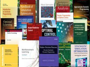
These problems are studied in at least 15 distinct fields, using eight different notational systems and a host of solution approaches. For years, I have been calling this the “jungle of stochastic optimization.” Each of these books (and associated communities) can be described as a method (or set of methods), and the problems for which these methods work. 

Sequential decision analytics turns this around; it is a field centered on the broad problem class of sequential decision problems, drawing on a broad class of methods (the “four classes of policies”) that span every solution approach that might be used.

There are four phases to addressing real-world sequential decision problems: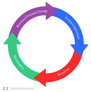

Phase I: Identifying the core elements of the problem (without mathematics):

• • Performance metrics – Costs, profits, yield, productivity, customer service, employee performance, …
  • Decisions – What types of decisions are being made, and who makes them.
  • Sources of uncertainty – We have to identify quantities and parameters we do not know perfectly when we make a decision, and the types of information that arrives after we make a decision.

Phase II: Developing the sequential decision model (turning the problem definition into math).  

• Developing the model – This requires defining the following five components:
  • State variables – This is all the information needed to compute the performance metrics, make decisions, and model the evolution of the system over time.  It includes information about physical and financial resources, other information, and beliefs about quantities and parameters we do not know perfectly.
  • Decision variables, including constraints.  We introduce the idea of a policy for making decisions, but defer to later designing the policy.
  • Exogenous information variables
  • The transition function, which models how the state variables evolve over time.
  • The performance metrics and objective function for evaluating policies.
• Modeling sources of uncertainty – This step is 

Phase III: Engineering – This is where we turn the model into software. The model might be used for strategic planning, or the much more difficult setting of operational planning.

Phase IV: Process change – Decision models require rethinking planning processes, especially when the model is being used for operational planning.  Process change typically reveals new elements of the problem that feeds back into the original problem defintion.

This page will focus on how to create a general mathematical model for sequential decision problems (Phase II).  Modeling is standardized in both deterministic optimization and machine learning, but not in stochastic optimization.  Sequential decisions represent a problem, which can be solved with a wide range of methods (that we will call policies).

The different communities of stochastic optimization are centered on methods which tend to be associated with problems for which the methods are well suited. I will show how to fix what I think is a major problem with the communities of stochastic optimization, which is the failure to standardize how problems are modeled.  This approach will separate the creation of the model from the design of policies for making decisions.

I will then show how my approach to modeling (which some use, but it is not common) creates a new approach for solving these problems that unifies all of the fields of stochastic optimization. By separating the model of the problem from the choice of policies for making decisions, I will open up the consideration of a much wider range of solution approaches.  In fact, I am going to present a universal framework that reduces every possible solution method into four (meta)classes of policies.  The four classes of policies will span any method that has been suggested in the research literature, as well as anything that might have been used in practice (when you see the classes, you will see why I can make such a broad claim).  In the process, I will highlight one method that has been largely ignored by the research literature, but widely used in practice.

It should be clear that the range of applications covered by sequential decision analytics is vast.  Yet, the academic community insists on researching (and teaching) the most complex policies that are rarely used in practice.  We should be teaching all four classes of policies, where we can guarantee that whatever a student does in practice, they will be using a policy drawn from one (or more) of these classes of policies.  This way, we allow them to choose the type of policy that works best for a particular situation.

In the process, I am going to highlight a new class of policy that is widely used in industry for certain problem classes which require planning into the future, but which has been almost universally overlooked by the research literature.  It is not a panacea (nothing is), but it is serious competition for any problem that can currently be approached using stochastic programming or model predictive control (that is, some form of lookahead policy).

Readers looking for much more depth into the ideas on this webpage are encouraged to explore the educational material at jungle.princeton.edu.  An online book used in my undergraduate course, Sequential Decision Analytics and Modeling, uses a teach-by-example style. A new book (in progress), Reinforcement Learning and Stochastic Optimization: A unified framework for sequential decisions (RLSO below), is being written entirely around the framework presented here.

Modeling sequential decision problems

To understand how we are going to model sequential decision problems, it helps to take a brief tour through two other major problem classes: deterministic optimization and machine learning.  We are then going to argue that our approach to stochastic optimization closely parallels the approaches these fields use.

Deterministic optimization models

Around the world the standard way of writing a linear program is

\min_x c^Tx,

subject to constraints which we might write

Ax = b, \\  x \geq 0.

To be a bit more general we might write the objective as

\min_x C(x)

where we might also insist that some or all of the vector x are integer. If we have a time-dependent problem (which is of particular interest to us), we might write

\min_{x_0,\ldots,x_T} \sum_{t=0}^T C_t(x_t)

subject to whatever constraints we need.

Note that we have written out different versions of a model, and we have not yet talked about how to solve the problem. It is absolutely standard in deterministic optimization to write out an objective function and constraints (the model), and then design an algorithm to solve it.  We call this “model first, then solve.” Sounds obvious, but it is not standard in stochastic optimization.

Machine learning

Now consider what happens when we are solving a machine learning problem.  Assume we have a training dataset (x^n,y^n)_{n=1}^N of input vectors x^n and responses y^n.  We want to find a function f(x|\theta) that minimizes some distance between f(x^n|\theta) and y^n over the entire training dataset.  We can be very general if we define a loss function L(x,y), but I will keep it simple by just assuming that we are minimizing the square of the difference.  We can write our objective function as

\min_{f\in F,\theta\in\Theta^f} \sum_{n=1}^N (y^n - f(x^n|\theta))^2

where F is a set of possible functions (“statistical models”) which might be linear or nonlinear in \theta, a nonparametric function, or a neural network.  If it is a neural network, f would describe the structure of the neural network (RNN? CNN?)  while the vector \theta would contain two types of information: the parameters governing the structure of the network (number of layers, number of nodes per layer), and the weights on the edges in the neural net (which can number in the millions).

The search over functions (statistical models) f\in F is often ad hoc.  An analyst has to choose functions from one of the three broad categories of functions: lookup tables, parametric models, and nonparametric models (see the figure – these are overlapping classes).  For example, a human may specify a linear model, and may even specify the input variables (aka basis functions), although a search algorithm may help with this.  Algorithms are always used to search for the best \theta.

Again, as with deterministic optimization, we have written out the objective function, and now we have to go find algorithms to find the solution.  Model first, then solve.

Monte Carlo simulation

There is an entire community known as the “simulation community” that works on a wide range of complex problems that have to be simulated.  These are typically motivated by the need to design a system: how to lay out a manufacturing plant; how to plan the capacity needed by a rail terminal; planning the performance of passenger flows through an airport.  These are not viewed as optimization problems, beyond the possible need to search over different configurations of the system being simulated.

Any sequential decision problem is just one step from a simulation problem.  All you have to do is to fix the policy X^\pi(S_t|\theta), and we now have a straightforward simulation problem.  In fact, searching over a set of policies is comparable to searching over different designs for our manufacturing system.

Anyone working in the field of stochastic models will end up using Monte Carlo simulation methods.  The simulation community created its own field called “simulation-optimization” to describe the tools for searching over different designs (such as the manufacturing configurations), but as a general rule this community has not tackled the problem of optimizing decisions within a simulator, such as policies for assigning ride-sharing drivers to customers, or optimizing inventories in a supply chain.

Sequential decision models

We are going to write our sequential decision model as consisting of state (what we know), decision, new information, state, decision, information, state, decision, … which we write as

S_0,x_0,W_1,S_1,x_1,W_2, \ldots, S_t,x_t,W_{t+1}, \ldots, S_T,x_T

Note that there are many settings where it is more useful to use a counter n than a time index.  We would write this as

S^0,x^0,W^1,S^1,x^1,W^2, \ldots, S^n,x^n,W^{n+1}, \ldots S^N,x^N.

There are even situations where we index by both time t (such as the hour of the week) and n (which might be the nth week).

There are five elements to any sequential decision problem:

• State variables S_t, which is the information available at time t needed to make a decision, compute costs/rewards, compute constraints, and provide any information needed to model the evolution of the system into the future.  State variables may describe the physical state of the system R_t, other (deterministic) information I_t,, and beliefs about uncertain quantities or parameters B_t.
• Decision variables x_t, which may be binary, discrete choices, or continuous or discrete vectors.  We require that x_t satisfy constraints so that x_t \in X_t at time t.  We also introduce the policy X^\pi(S_t|\theta) where we have to design the policy to ensure that X^\pi(S_t|\theta) \in X_t, but we defer designing the policy to later.
• Exogenous information W_{t+1}, which is the information that arrives after we make decision x_t but before we make decision x_{t+1}.
• Transition function S_{t+1} = S^M(S_t,x_t,W_{t+1}) which describes how the decisions and exogenous information updated all the elements of the state variable.  Note that the transition function (this goes by many names in the literature, including system model and plant model) can be hundreds, even thousands, of lines of code.
• Objective function, which can come in different forms but a standard one is

max_\pi \mathbb{E} \left\{\sum_{t=0}^T C(S_t,X^\pi(S_t))|S_0\right\}

where C(S_t,x_t) is the contribution that we receive when we make decision x_t given the information in state S_t.  There are different variations of objective functions depending on whether we are maximizing cumulative rewards (the form we have chosen) or final reward (we may be sequentially optimizing a process offline).  We may use expectations, risk metrics or worst case (as is done in robust optimization).

[Side note: our framework closely parallels that used in optimal control, but with some differences.  For a comparison of frameworks, click here.]

A simple way of stating a sequential decision problem that parallels that used for deterministic optimization would be to write the objective function

max_\pi \mathbb{E} \left\{\sum_{t=0}^T C(S_t,X^\pi(S_t))|S_0\right\}

given the transition function

S_{t+1} = S^M(S_t,x_t,W_{t+1}),

and given an exogenous information process

S_0,W_1,W_2, \ldots, W_t, \ldots, W_T,

which may come from a mathematical model (if we are simulating), history, or live observations from the field.

Once this model is given, there are two major elements we have to specify:

• The uncertainty model.  This starts with S_0 where we may have to specify beliefs or priors about uncertain quantities, followed by a process for generating W_1,W_2, \ldots, W_T.  Uncertainty modeling, also known as uncertainty quantification, is often viewed as being more important than optimizing policies.
• Designing the policy X^\pi(S_t|\theta).  Unlike deterministic problems where we want to choose x_t,  we want the best function which returns a decision given a state. We let \pi = (f,\theta) carry the type of function f\in F and any tunable parameters \theta\in\Theta^f (just as is done in machine learning).  The search over policies \pi can also be written as

\max_{\pi=(f\in F,\theta \in \Theta^f)} \mathbb{E} \left\{\sum_{t=0}^T C(S_t,X^\pi(S_t|\theta))|S_0\right\}

So, our deterministic optimization problem which optimizes over x_0, \ldots, x_T becomes a search over policies (or functions) for making decisions X^\pi(S_t|\theta).  Many people find this confusing which is why we think the communities working on these problems have become fragmented into different types of policies, but it is really no different than what is routinely done in machine learning.  What is different is the set of functions is much richer, and some are much more complex.

An illustration of this way of modeling problems is the online book here.  The book, which uses a teach-by-example style, was used in an undergraduate course at Princeton.

We are going to return to the problem of searching over policies, but first we are going to briefly stop to consider the oldest problem in stochastic optimization that is often given the name “stochastic search.”

Stochastic search

The fundamental problem of stochastic search, dating back to 1951, is written

\min_x E f(x,W)

where W is a random variable. This seems much more familiar, since we are optimizing over x just as we did in deterministic optimization.  In fact, this problem, as written, is a deterministic problem (if we can compute the expectation), and expresses the desire of finding the optimal solution (a deterministic quantity).

The problem is, we never do this.  Instead, we almost always end up with some form of adaptive learning algorithm that takes a point x^n at iteration n, along with other information, to make another guess x^{n+1}.  This algorithm actually works just like a policy.  If we let S^n be the data we need after n iterations to compute x^{n+1} (think of S^n as the “state of the algorithm”), we can write our algorithm as a policy using

x^n = X^\pi(S^n|\theta)

where \theta captures any tunable parameters we might need.  We then observe our function F(x^n,W^{n+1}), update our beliefs about F(x) = E f(x,W) which produces an updated (belief) state S^{n+1}.

Next remember that despite the vast literature on asymptotic convergence proofs (a number written by me and my students), we never run algorithms to infinity.  If we run N iterations, we would obtain a solution we represent by x^{\pi,N} to represent that the solution depends on our policy (algorithm), but also on the number of iterations N.  Also keep in mind that x^{\pi,N} is a random variable.  We can now state our optimization problem as

\min_\pi \mathbb{E} F(x^{\pi,N},W)

This objective function says that we want the best algorithm in terms of getting the best solution (in expectation) after N iterations.  So, we are back to optimizing over policies.  Since our “policy” here is an algorithm, what we are really doing is looking for an optimal algorithm, or at least we want to optimize within a class of algorithms (think of this as tuning stepsize rules).

Stochastic search arises frequently in policy search when we have a parameterized policy, and have to look for the best value of the parameters that characterize the policy.  In this case, we have to solve a sequential decision problem (the search algorithm) to solve a sequential decision problem (tuning a policy to make decisions in our real application).

We note that both machine learning and stochastic optimization require optimizing over functions.  However, the machine learning community recognizes this, and virtually every book on machine learning will describe a variety of models (functions), so that students trained in machine learning can choose from a family of models.  This is absolutely not the case in stochastic optimization, where students typically learn a very small number of policies reflecting the community of the faculty member teaching the course.

Some notes on notation

When developing a modeling framework, you have to choose a notational system.  Below are some brief comments explaining my choices:

• Decisions – The field of math programming is so large, and so established, and so … useful… and it uniformly uses x for decisions, where x can be binary, a member of a discrete set, continuous or discrete vectors.  In other words, anything.  There are two other standard notations for decisions: a for discrete actions, used in Markov decision processes and adopted from there by the rapidly growing reinforcement learning community.  However, a is almost always a discrete action.  The controls community uses u, where u is typically low-dimensional (think of force in three dimensions) and continuous.  If you have a problem with discrete actions, I think a is fine, but I would note that the bandit community, centered in computer science, uses x for discrete arms (but where x can be continuous, or even a vector).
• The controls community (which is very large) likes x for state, which conflicts with our choice of x for decisions.  Also, there are large communities in dynamic programming that think s, or S, should be state.  Seems natural.
• The only community with standard notation for information (I use the term exogenous information) is the controls community which uses w_t for information.  In continuous time this is the information arriving between t and t+dt, so many authors translate this for discrete time to the information arriving between t and t+1.  This means w_t is random at time t, which can create a lot of confusion.  After consulting different colleagues (but esp. the renowned probabilist Erhan Cinlar), I decided to use W_{t+1} for the information that first becomes available at time t+1 (said differently, the information arriving between t and t+1).  In my notation, any variable indexed by t is known at time t.
• The only community that routinely uses the concept of a transition function (although this is described by many names) is the controls community that typically would write (using controls notation) x_{t+1} = f(x_t,u_t,w_t).  The letter f is incredibly useful for defining a range of functions.  I decided to go with S_{t+1} = S^M(S_t,x_t,W_{t+1}) where S^M(\cdot) stands for “system model” or “state transition model,” which avoids taking up another letter in the alphabet.

Back to the jungle

Above, we have a picture with the front covers of books representing at least 15 distinct fields that all deal with some form of stochastic optimization.  Bizarrely (for an optimization field) is the lack of formal statements of an objective function which means optimizing over a set of policies (even a set of policies within a class), as well as how a policy is being evaluated.

The reality is that virtually every book in the “jungle of stochastic optimization” provides a framework that focuses on describing a policy rather than the kind of proper model (objective function with constraints) that is absolutely standard in deterministic optimization (as well as machine learning).

What differentiates these fields of stochastic optimization is:

o The nature of problems that each field works on.
o The type of policies that each field develops and promotes.

The challenge we now face is… how do we optimize over policies?

Designing policies

We are going to search over policies by standing on the shoulders of the entire body of research in the jungle.  However, rather than say something useless like “try everything in all those books,” we are going to observe that every approach can be divided into two broad classes (the policy search class, and the lookahead class), each of which can be further divided into two subclasses, creating what we have been calling “the four classes of policies” (try searching on this term). Sadly, we do not have a magic wand in the form of a single policy that solves all problems (although I have met people who claim to have done so), but reducing all those fields into these four classes greatly simplifies the search.  We also note that one of the four classes is new to the research literature, but popular in practice. We return to this policy later.

The four classes of policies are:

• The policy search class – These are functions with parameters that have to be tuned to find the values that work best over time, averaged over all the possible sample paths. This class consists of two sub-classes:
  • 1) Policy function approximations (PFAs) – These can be simple rules, linear functions, nonlinear functions (such as neural networks) and nonparametric functions.  PFAs include every possible function that might be used when we are searching for statistical models for machine learning.
  • 2) Cost function approximations (CFAs) – We can take a simplified optimization model and parameterize it so that it works better over time, under uncertainty.  CFAs are very popular in engineering practice, but virtually ignored in the stochastic optimization community.
• The lookahead class – This policy makes better decisions by estimating the downstream value of a decision made now. This class also has two sub-classes:
  • 3) Policies based on value function approximations (VFAs) – This is the class (and the only class) that depends on Bellman’s equation (also known as the Hamilton-Jacobi equations in control theory). It creates policies by optimizing the first period contribution (or cost) plus an approximation of the value of the state that a decision takes us to.
  • 4) Direct lookaheads (DLAs) –
  • These are where we plan over some horizon using an approximate lookahead model.  Unlike VFA-based policies, we explicitly optimize over decisions we may make in the future. DLAs come in two broad flavors:
    1. Deterministic lookaheads – This is easily the most widely used strategy in transportation and logistics.  Often overlooked is that deterministic lookaheads can be parameterized, creating a hybrid DLA/CFA (CFAs are parameterized optimization problems, but a vanilla CFA does not plan into the future).  Navigation systems (such as google maps) are a classic example of a deterministic lookahead.
    2. Stochastic lookaheads – These come in many forms.  One of the best known in the operations research community for problems in transportation and logistics is stochastic programming (notably two-stage stochastic programs) first introduced by Dantzig in 1955 for a transportation problem involving aircraft.

In addition to these four classes, we can create a variety of hybrids:

• Tree search terminated with value function approximations (DLA with VFA).
• Deterministic lookahead, parameterized to make it perform better under uncertainty (DLA with CFA).
• Monte Carlo tree search, which is a stochastic lookahead (DLA) with a rollout policy (which might be a PFA), exploration strategy (CFA, using upper confidence bounding) and value function approximations (VFA).
• Any optimization-based policy (CFA, VFA or DLA) with rule-based penalties (PFA).

At the end of the day, if you have a sequential decision problem, you need a method for making decisions and any method you use will belong to one of the four classes (or a hybrid).  The four classes are universal.

Some notes:

• Any of the four classes of policies can produce optimal (possibly asymptotically optimal) policies, at least for specific problem classes.
• The policy search classes are simpler than the lookahead classes, with the single exception of deterministic DLAs (when they are appropriate).  But… the price of simplicity is tunable parameters, and tuning can be hard (see below).
• PFAs include the same classes as machine learning: lookup table, parametric (linear and nonlinear, including neural networks), and nonparametric.  This means the remaining three classes of policies are unique to decision making.
• The remaining three policy classes (CFAs, VFAs and DLAs) all have imbedded optimization operators, which means they are able to handle high-dimensional actions.  Once you have an optimization problem, you can use any of the solvers for linear, integer and nonlinear programming problems.
• PFAs, CFAs and VFAs all involve some form of machine learning.  DLAs may involve machine learning, but not necessarily.
• DLAs may be parameterized deterministic lookaheads (which involves learning), or some form of stochastic lookahead, which almost always involves solving an approximate lookahead model. There are seven classes of approximations when creating an approximate stochastic lookahead, one of which involves coming up with a policy within a policy (see chapter 20 of RLSO).
• The policy search policies are always simpler which reflects their wide popularity, but the price of simplicity is tunable parameters, and tuning is hard.  Tuning can be done offline in a simulator, or online in the real world.  The latter is much harder, but simulators may introduce modeling approximations.  For the algorithmic research communities, there are fabulous challenges here.
• Tunable parameters will also arise in DLAs when approximations are used (which is virtually always the case).  Tuning a DLA in a simulator (the most common way for tuning to be performed) can be computationally demanding.
• An optimal solution of an approximate stochastic lookahead (such as stochastic programming) is not an optimal policy.  Bizarrely, I have met leaders in the field who do not understand this simple point.

It is important to emphasize that the four classes of policies are meta-classes.  Just picking one of the four classes (or a hybrid) does not mean your problem is solved, but it should help highlight different avenues to pursue.  Particularly important is that by recognizing all four classes brings greater visibility to all the research in the field.

Academics doing algorithmic research prefer the more challenging classes, specifically VFAs (this is where you find approximate dynamic programming and most of reinforcement learning) and DLAs with some form of stochastic lookahead. People working on an application, however, typically want something simple, which means PFAs, CFAs, and deterministic DLAs. As academics, we need to expose students to the entire spectrum of policies so that they can make a more intelligent choice when they have to choose a method for making decisions.

I am frequently asked how I know which class to use.  This is one of those questions where theory (at the moment) is of little help.  You have to have a feel for the empirical characteristics of a problem, and the capability of different approximation architectures.  For example, a simple buy low, sell high rule is an effective PFA for purchasing stocks (or energy), but you would never use a PFA to find the best path through a network.  At the bottom of jungle.princeton.edu, I describe a paper (joint with Stephan Meisel) on the control of an energy storage problem where we show that by tweaking the data, we can make each of the four classes of policies work best!

We believe that the academic community needs to learn to teach students a standard modeling framework, such as that proposed here, just as is done in deterministic optimization and machine learning. The model should not presume a particular policy for solving it. Then, we need to cover all four classes of policies, just as texts on machine learning provide a balanced overview of statistical models.

Tuning policies

While the academic research community has focused most of their attention on policies in the lookahead class, the real world has primarily been using policies in the policy search class (with some use of deterministic DLAs, but these can be parameterized as well).  Policy search policies are simpler, which suggests they are somehow less interesting, but there are some compelling arguments for simplicity (ease of development, ease of computation, transparency, diagnosability), and they may even work better for problems where there is apparent structure that can be exploited.

But as we said above, the price of simplicity is tunable parameters, and tuning can be hard.  What often happens in practice is that a developer will pick what seems to be reasonable values for the tunable parameters, and just leave it there.  If you are not tuning your tunable policy, then you are not doing stochastic optimization.

The most natural way to perform tuning is through a simulator, which means we have a set of equations to represent the transition function.  Now, pick a form of parameterized policy. Some examples are:

• Buy when the price goes below \theta^{min}, sell when it goes above \theta^{max}.
• When planning a path using a navigation system, add a buffer \theta^{slack} to the trip, which can be adjusted after you complete each trip.
• When optimizing the assignment of truck drivers d to loads \ell of freight that have been waiting, minimize the modified cost C(S_t,x_t|\theta)=\sum_{d} \sum_{\ell} (c_{tdl} - \theta \tau_{t \ell}) where \tau_{t \ell} is how long a load has been held, and \theta is the penalty placed on waiting.
• We are learning the performance of different drugs x \in {x_1,x_2,\ldots,x_M}.  Let {\bar \mu}^n_x be the estimate of the performance of drug x after n experiments and let {\bar \sigma}^n_x be the standard deviation of our estimate {\bar \mu}^n_x.  Choose the next drug to purchase by solving the (simple) optimization problem \max_x ({\bar \mu}^n_x + \theta {\bar \sigma}^n_x).  This is a rare parametric CFA with provable properties, mostly in the form of regret bounds but there are also some asymptotic results.

Each of these are examples of a policy with a tunable parameter \theta.  The most common objective function that we would use to optimize \theta (but not the only one) is

\max_{\theta \in \Theta^f} F(\theta) = \mathbb{E}\left\{\sum_{t=0}^T C(S_t,X^\pi(S_t|\theta))|S_0\right\}

Since we cannot compute the expectation, we have to turn to stochastic search algorithms which might be derivative-based or derivative-free.  These are discussed in chapter 5 and chapter 7, respectively, of RLSO  . Note that both derivative-based and derivative-free stochastic search algorithms are, themselves, sequential decision problems.  This issue is not emphasized for derivative-based methods in chapter 5, but it is central to the presentation for derivative-free methods in chapter 7.

For people looking for practical solutions to problems, PFAs and CFAs (and sometimes deterministic DLAs) will represent the simplest policies.  Of particular value is that they allow a knowledgeable user to exploit intuition about the structure of the problem.  However, tuning can be hard, and not all problems have obvious structure to exploit.  One challenge is developing a simulator, and in many settings simulators are expensive to develop.  An alternative is to use online learning, such as setting the amount of time to leave early on a trip based on your past experiences with the same trip.  However, online learning can be quite slow (it takes a day to simulate a day) and you have to experiment in the field.

The classes of policies and the jungle

Each of the communities in stochastic optimization started with one algorithmic strategy, often motivated by a small class of applications that fit the method.  However, as time has passed and the communities have grown, so have the range of problem classes they are working on.  Then, as the characteristics of the problems have evolved, the communities have found that the original methods no longer work (there are no panaceas in this field), and as a result they have explored policies from other classes.

The figure below illustrates the evolution of seven major fields (labeled in the seven outer ovals) from one or two of the four classes of policies (represented as rectangles in the middle).  Wider white arrows indicate the initial policy used by the field, with narrower lines indicating the evolution to policies from the other classes.  A number have grown to use examples from each of the four classes, but not all (see stochastic programming).  What is missing, however, is the use of a standard framework (which we present above) of optimizing over policies, ideally from across the four classes.

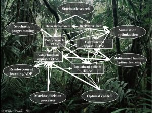
Below is a discussion of some of the evolutions of different fields:

• Stochastic search traces its roots to two papers in 1951 – one for derivative-based stochastic search, and one for derivative-free stochastic search.  Derivative-based stochastic search can be presented as a sequential decision problem where the decision is the stepsize, almost always determined with a parameterized stepsize rule (a PFA).  However, derivative-free stochastic search has quickly evolved to using all four classes of policies.
• Simulation-optimization – This community originally focused on evaluating competing configurations for manufacturing systems using a DLA called optimal computing budget allocation (OCBA).  A few years ago Michael Fu came out with “Handbook of Simulation Optimization” that covers many of the major topics in stochastic optimization using all four classes, but never formalizes the process of searching over all four classes.
• Multi-armed bandit problems – These are active learning problems where we try discrete alternatives to improve our understanding of how well it works.  It started in the 1970s with a breakthrough known as “Gittins indices” which is based on solving Bellman’s equation (a VFA), then transitioned to upper confidence bounding in the 1980s (a CFA).  Today, all four classes of policies are used. [Multi-armed bandit problems are all a form of derivative-free stochastic search.]
• Optimal control started with Hamilton-Jacobi (that is, Bellman) equations, which is a VFA, but was able to show for a class of problems known as “linear quadratic regulation” that the policy reduced to a linear function (a PFA).  In the 1970s Paul Werbos learned how to use backpropagation to approximate value functions (a VFA).  Finally, there is an entire subfield in optimal control called model predictive control (MPC), which is a deterministic lookahead (a DLA).
• Markov decision processes evolved originally using Bellman’s equation using discrete states (lookup table VFAs), which is a VFA-based policy, although special cases were found that produced analytical solutions to policies (PFAs).  However, the curse of dimensionality that arises with lookup table representations motivated the use of approximate dynamic programming, which is all VFA-based, but the research literature also explored the use of parameterized policy (PFAs).
• Reinforcement learning in the 1990s and early 2000s was limited to Q-learning (see the discussion on what is reinforcement learning here), as presented in the first edition of Sutton and Barto’s now classic Reinforcement Learning: An Introduction.  But if you compare this edition to the second edition (2018), the range of methods has expanded to include a variety of other algorithmic strategies (parameterized policies (PFAs), upper confidence bounding (a CFA), Q-learning (a VFA) and Monte Carlo tree search (a stochastic DLA).  These are samples drawn from each of the four classes, but there the field has never formalized the process of searching over all four classes to find which one is best.
• Stochastic programming was initiated by George Dantzig in the 1950s using scenario trees, which is a form of stochastic DLA, but in the 1990s the research community developed “stochastic dual dynamic programming” (SDDP) which is a form of approximate dynamic programming using Benders cuts to approximate convex value functions (a VFA-based policy).  SDDP may be a stochastic lookahead – it depends on how the model is being used (this is true of all ADP-based applications).

Introductory tutorial 

For an introduction to the unified framework: I revised and re-recorded a tutorial on the unified framework that I gave at the Kellogg School of Business at Northwestern (February 2020).  It is now on youtube in two parts:

1. Describes applications, the universal modeling framework, and introduces the four classes of policies for making decisions in the context of pure learning problems (derivative free stochastic search, also known as bandit problems). Click here for slides to Part I.
2. Here I illustrate the four classes of policies in the context of more general state-dependent problems.  I then briefly illustrate how these ideas are used at Optimal Dynamics. Click here for slides to Part II.

•  

Teaching sequential decision analytics

I believe that sequential decision analytics is a field that should be taught alongside courses in optimization and machine learning.  This can be done in several ways:

An undergraduate course – I taught a course at Princeton spanning a wide range of applications, using a teach by example style.  See the lecture notes and an online book. However, this is a course that is easily adapted to any problem domain just by creating different illustrative examples.

A graduate level course – I taught this material at the graduate level, although to a broad audience (eight different departments), with more emphasis on methodology. My lecture notes are available and I am working on a graduate level book.

Alternatively, this material can be inserted in courses that need this material, but where you do not have enough time to devote more than 2-4 lectures.  I suggest using the online book I wrote for the undergraduate course.  You can teach the modeling style using a simple example of your choosing, and then re-enforce the ideas through additional examples relative to the course.  The challenge is that it is nice to illustrate different classes of policies, as I do in chapters 2-6 of the online book.

The parametric cost function approximation

The parametric cost function approximation emerged while putting this framework together. I came to appreciate it while working in energy, and then started to realize how powerful it could be in many settings.

It is an idea that is widely used as an engineering heuristic, but disregarded (and largely discounted) by the academic research community in stochastic optimization. I believe, strongly, that this has been a major oversight.  Given the importance of the idea, I have created a page dedicated to the idea.