Warren B. Powell
Professor Emeritus, Princeton University
Chief analytics officer, Optimal Dynamics
Within the vast class of problems that fall under the umbrella of sequential decisions (decision, information, decision, information, …) there are many problems that naturally call for policies that plan into the future in order to decide what to do now. Some examples are:
- Deciding the next turn while planning a path to a destination over a road network.
- Planning which energy generators to have running tomorrow to meet energy demand given the uncertainty in wind, solar and temperature.
- Managing the flows of water between reservoirs given current forecasts of rainfall.
- Routing a fleet of vehicles making pickups and/or deliveries as orders arrive dynamically.
- Scheduling machines to meet order deadlines, with new orders arriving randomly.
- Managing the inventory of high value products to meet scheduled demand requests.
These can be complex problems without having to deal with uncertainty, but all of these examples require making decisions in the presence of different forms of uncertainty: demands, weather, travel times, equipment failures, …
There are a number of complex, sophisticated tools that have been proposed in the academic literature for these problems that explicitly handle uncertainty, but very little of this work is actually used in practice. Notable is the whole approach used in two-stage stochastic programs that depend on scenario trees. In fact, I recognized the power of this approach when I became involved in one of the most popular problems in stochastic programming, the stochastic unit commitment problem. For a discussion of this problem and the limitations of stochastic programming, click here.
This webpage will introduce a new approach, called a parametric cost function approximation, that formalizes a widely used industrial heuristic which is not just practical, but which may even outperform much more complex methods found in the academic literature. The core idea is to parameterize a deterministic model, and then to optimize the parameterization. What is missing in industrial applications is the tuning, which requires formulating the tuning problem as a stochastic optimization problem.
This idea (and hence this webpage) should be of interest to two communities:
- People focusing on applications where you need to optimize problems (such as those above) over time in the presence of different forms of uncertainty, where you are particularly interested in using a deterministic lookahead policy (some call this “model predictive control”).
- Algorithmic specialists looking for a nice challenge. In particular, parametric CFAs represent the bridge between machine learning and stochastic programming. While a parametric CFA is easy to implement, there are difficult algorithmic challenges that parallel problems such as fitting neural networks to large datasets.
The challenge of planning under uncertainty
All of these problems require planning into the future to determine what decision to make now. Given the different forms of uncertainty (travel times, customer demands, rainfall, product yields, prices, performance of vaccines, …), we should be capturing this uncertainty as we plan if we want to make the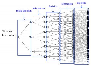 best decision now. The problem is that planning under uncertainty is hard.
The figure to the right illustrates the familiar explosion of a decision tree, and this is for a very simple problem (e.g. three possible decisions each time period). Bellman’s introduction of Markov decision processes was a breakthrough for these problems, but this has been restricted to small (even toy) problems because of the infamous “curse of dimensionality” (there are actually three curses).
Now imagine we are managing a fleet of 1000 vehicles where we may have a decision vector with 10,000 dimensions. In the 1950s, George Dantzig introduced the idea of using a lookahead policy where the uncertainties in the future are represented through a small sample (his motivating application was in scheduling airlines). This idea created the field of stochastic programming, which has produced thousands of papers and a number of books. If we let \Omega_t represent a sample of outcomes (demands, deviations from wind forecasts, travel times, equipment failures), then we could make a decision using
X^\pi(S_t) =\argmax_{x_t}\left(c_tx_t + \sum_{\omega\in\Omega_t}p_t(\omega)\max_{x_{t,t+1}(\omega),...,x_{t,t+H}} \sum_{t'=t+1}^{t+H} c_{t'}(\omega)x_{t'}(\omega)\right) (1)
subject to some constraints for the decision to be made now, x_t, as well as the decisions that would be made in the future x_{tt'}(\omega) for each scenario \omega\in\Omega_t.
This optimization problem is much larger than a method that just uses point estimates of the future, as is done with navigation systems that use a point estimate of travel times over each link in a network. There are many problems where some or all of the variables have to be integer; introducing scenarios in the lookahead model can make these problems exceptionally difficult.
What is often overlooked is that even when we can solve a stochastic program within computational constraints (a major issue in many applications), an optimal solution to a stochastic program is not an optimal policy, because a number of approximations have been made in the lookahead model. Some of the most significant include:
- The replacement of a fully sequential decision problem in the future. Ideally, we want to make decision x_{t,t+1}, observe information W_{t,t+2}, make another decision x_{t,t+2}, observe information W_{t,t+3} (and so on). With the two-stage approximation used in the stochastic program above, we assume we first observe all the information \omega = (W_{t,t+1}, W_{t,t+2}, \ldots, W_{t,t+H}) and then make all the decisions x_{t,t+1}(\omega), x_{t,t+2}(\omega), \ldots, x_{t,t+H}(\omega). This means x_{tt'}(\omega) gets to “see” W_{t,t'+1}(\omega), W_{t,t'+2}(\omega), \ldots, which means decisions starting at time x_{t,t+1} are allowed to see the entire future.
- Replacing all outcomes with a sample.
- Stochastic outcomes in the future have to be independent of any decisions (at time t or later).
- Limiting the horizon t,t+1, \ldots, T with the truncated horizon t,t+1,\ldots,t+H.
- Often other approximations are made in the future, such as discretizing time periods (say, into hours instead of minutes, or days instead of hours).
Stochastic programming has attracted considerable attention from the research community, but very little of this work has been implemented in practice, for several reasons:
- The stochastic program is complicated!
- It is hard to solve, requiring computation times that may be far beyond what can be tolerated in practice.
- The analyst has very little control over how the resulting policy responds to uncertainty, while in practice, practitioners often have very good intuition about how they want to deal with uncertainty.
The parametric cost function approximation
The most common approach used in practice is to solve a deterministic model, but introduce parameters to improve robustness of the solution. Examples include:
- We may use the shortest path from the deterministic model, but we leave \theta = 10 minutes earlier than the deterministic model recommends so we arrive on time.
- We plan our energy generator for tomorrow, but introduce a vector \theta of reserves in different regions of the network, taking known bottlenecks in the grid into account.
- We plan the flow of water between reservoirs, but introduce upper and lower limits, captured by a vector \theta that keep the system from allowing reservoirs to get too low or too high. This makes it possible to draw down even when the reservoirs are at their lowest level if there is less rainfall than expected, or to store more if rainfall is more than expected.
- Scheduling vehicles or machines to perform tasks, but introducing slack \theta in the time required to complete certain tasks in case of equipment issues.
The use of deterministic models with tunable parameters \theta has been a widely used engineering heuristic, which has been largely dismissed by the academic community as nothing more than a deterministic approximation. Many who work in stochastic programming assume that introducing scenarios automatically means that these models are better, but these claims are made with virtually no empirical evidence (and certainly no theoretical support, given the approximations required by stochastic programming).
Tunable parameters can be introduced as adjustments to the objective function, or (more often) as changes to constraints. We can write this in a generic way as
X^{\pi}(S_t|\theta) = \argmax_{x_t=(x_{tt}, \ldots, x_{t,t+H})} {\bar C}^{\pi}(S_t,x_t|\theta) (2)
subject to
x_t \in X_tWe can parameterize the objective function, and/or the constraints.
The central idea here is to parameterize a (typically deterministic) optimization model, which creates two challenges:
- How do we parameterize the optimization model? This work belongs in the context of the motivating application, since it draws on insights into the structure of the particular application. The issues are comparable to the design of any parametric model in statistics, but (we believe) the opportunities are much richer.
- Tuning the policy X^{\pi}(S_t|\theta) – This is a purely algorithmic exercise which offers a number of fresh challenges in context of parameterized optimization problems, just as neural networks have introduced fresh challenges for parameter search while fitting neural networks to datasets.
Designing the parameterization
As with any parametric model, the structure of the parameterization is more art than science (as of this writing). Parametric models date back to the early 1900s in the statistics community. Easily the most popular form of parametric model is a model that is linear in the parameters, which we might write as
Y = \theta_0 + \theta_1 \phi_1(x) + \theta_2 \phi_2(x) + \ldots + \varepsilonwhere \phi_f(x), f\in F is a set of features (also known as “basis functions”) that depend on an input dataset x. We could use this idea to modify our objective function, giving us
{\bar C}^{\pi}(S_t,x_t|\theta) = C(S_t,x_t) + \sum_{f\in F} \theta_f \phi_f(S_t,x_t)Here, the additional term \sum_{f\in F} \theta_f \phi_f(S_t,x_t) could be called a “cost function correction term,” and requires carefully chosen features \phi_f(S_t,x_t).
The most common way to parameterize constraints would be through the linear modification of the right hand side, which we can write as
A_t x_t = \theta^b \otimes b_t + \theta^cwhere \otimes is the elementwise product of the vector \theta^b times the similarly dimensioned vector b_t, and \theta^c is a set of additive shifts.
Adding schedule slack would require parameterizing the A_t matrix. We can also shift upper and lower bounds on x_t.
Tuning the parameterization
However you design the modified objective function, we then face the problem of tuning \theta. This is its own optimization problem, which we might write as
max_\theta F^\pi(\theta) = \mathbb{E}\left\{ \sum_{t=0}^T C(S_t,X^\pi(S_t|\theta))|S_0\right\} (3)
where the evolution of the state variable is determined by
S_{t+1} = S^M(S_t,X^\pi(S_t|\theta),W_{t+1})and given by an underlying stochastic model for generating the sequence
W_1(\omega), W_2(\omega), \ldots, W_T(\omega).We refer to this as the stochastic base model, which is typically implemented as a simulator, but there are settings where we are optimizing the policy in the field.
The first question we have to answer is: how are we going to evaluate the policy? We are going to need to run a simulation, but there are two ways to do this:
- Simulating the policy in the computer. Here, there are two ways of generating the exogenous information process W_1, \ldots, W_t, \ldots:
-
- Sampling from a stochastic model
- Using sequence of observations from history (often called backtesting).
-
- Testing in the field – This can be very slow (it takes a day to simulate a day), but it avoids any of the modeling approximations of Monte Carlo simulation. Typically this means that we have to learn by doing, which means that we have to live with our outcomes (this is called optimizing cumulative reward).
While we can do much more with a simulation model, these can be time-consuming and expensive to build, in addition to the fact that we still have to live with modeling approximations. Testing policies in the field is what is done most often in practice, but often without any formal process of learning and improving.
This is a classical stochastic search problem, which can be approached using two basic approaches:
- Derivative-based stochastic search – See chapter 5 of Reinforcement Learning and Stochastic Optimization.
- Derivative-free stochastic search – See chapter 7 of Reinforcement Learning and Stochastic Optimization.
Note that you can only do derivative-based search in a computer-based simulator.
The difference between our parameterized CFA, and standard industry heuristics, is the formal statement of the objective function for tuning the parameters, which is the basis for any stochastic search algorithm. For example, we have never seen a formal statement of an objective function for a policy based on stochastic programming. People will formulate the stochastic program (which is just a form of lookahead policy), but do not realize that this is just a policy that has to be simulated to be evaluated. By contrast, the objective function F^\pi(\theta) is central to the parametric CFA policy, just as an objective function is central to the design of any search algorithm in deterministic optimization.
An important property of a parametric CFA is that it will typically be the case that the coefficient vector is inherently scaled. At the bottom of this page, we present a case study where the parameter vector \theta is centered around \theta = 1. It uses rolling forecasts, and if the forecasts happen to be perfect, then the optimal value of \theta satisfies \theta = 1. This would not be the case if we were using, for example, a linear model or neural network.
From stochastic lookaheads to stochastic base models
It is very common in the algorithmic community to view a stochastic lookahead as the gold standard. The problem is that stochastic lookaheads are inherently complicated, as hinted by the exploding scenario tree above. The stochastic programming community has learned to live with the different approximations this approach requires. For example, there may be arguments about how many scenarios \Omega_t are required, but rarely is there a debate about the use of two-stage approximations, since three-stage models are almost always unsolvable. They do not even raise the possibility of modeling every time period in the future as its own stage.
The process of tuning the parametric CFA, on the other hand, focuses on putting the stochastic model in the simulator required to evaluate F^\pi(\theta). While putting complex dynamics in a lookahead model is quite difficult, it is comparatively easier in the simulator captured by the transition function S_{t+1} = S^M(S_t,X^\pi(S_t|\theta),W_{t+1}). This means that the tuned value of \theta has these complex dynamics captured by the optimal solution \theta^*.
For this reason, we claim:
A properly designed and tuned parametric CFA may easily outperform a much more complex stochastic lookahead, such as those produced by stochastic programming.
It is important to emphasize that no policy, including parametric CFAs, is a panacea. The universe of sequential decision problems is simply too vast. However, the types of problems that are good candidates for stochastic programming (regardless of whether you are using scenario trees or SDDP) are likely to be good candidates for parametric CFAs.
There are many papers that formulate stochastic programs to solve a sequential decision problem, which do not then run simulations, but there are some that do. The most common competition is to compare a stochastic lookahead (using scenario trees) against a “deterministic model.” These comparisons never compare against a properly parameterized and tuned deterministic model.
A case application
We have demonstrated this idea in a complex form of energy storage application. The energy system consists of four elements: energy from the grid, energy from a wind farm, a storage device, and a load (demand) for energy: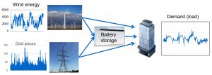
There is a demand for energy that follows a consistent hour-of-day pattern (figure below on the left), along with rolling forecasts of wind that are updated hourly (figure on the right).
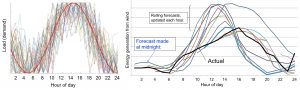
These two types of variability are different in an important way. The time-of-day demand pattern means that the high and low points occur consistently at the same time of day, which could be picked up with a parameterized policy where the parameter \theta_t is indexed by time.
This is not the case with the rolling forecast, where the peak wind forecast can change over time, as it does in the illustration of forecasts in the figure on the right. In this figure, black is the actual wind (observed at the end of the day), while the other lines are forecasts made each hour, where the peak wind changed over the course of the day. If f^W_{tt'} is the forecast of wind for hour t' made as of hour t, then the vector of forecasts f^W_t = (f^W_{tt'}), t'=t, ..., t+24 has to be treated as part of the state variable. See here (section 5) for a proper model of rolling forecasts for this energy storage problem.
[One way to solve this problem using a stochastic lookahead model would be to make the forecast a latent variable, which means we model the errors in the forecast, but otherwise lock the forecasts in place and treat them as constants (this means we are not modeling the fact that these forecasts are evolving over time). Imagine that we solve this stochastic model using approximate dynamic programming, which means that we have to estimate value function approximations {\bar V}_t(S_t) where S_t might capture how much energy is stored in the battery, but does not include the current set of forecasts f^W_t. This means that when we step from t to t+1, we would have to re-estimate the value functions {\bar V}_t(S_t) entirely from scratch.]
A powerful way to handle both the time-of-day effect, as well as the rolling forecast, is to use a deterministic lookahead model, parameterized by introducing coefficients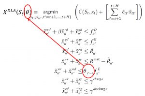 \theta_\tau for \tau=1, 2, ..., 24 in front of each forecast f^W_{t,t+\tau}. The resulting policy is a simple linear program given by the figure to the right. This policy is no more complicated than a simple deterministic lookahead, obtained by setting \theta_\tau = 1 for all \tau.
This lookahead policy is both stationary, and has the current forecast imbedded in the policy. Of course this means that we have to re-optimize the deterministic lookahead as the forecasts change, but this is extremely fast (a fraction of a second).
Using this policy in the field is very easy. Tuning the parameter vector \theta, however, is not. We used a stochastic gradient algorithm based on Spall’s simultaneous perturbation stochastic approximation (SPSA) method, which allows us to estimate an entire gradient with just two function evaluations. However, our simulations were extremely noisy, which meant that we had to perform “mini-batches” of perhaps 20 simulations which were then averaged. Also, the objective function F^\pi(\theta) is nonconvex, but appears to be unimodular. Please click here for a paper summarizing our work on tuning the policy, which produced results 30 to 50 percent better than a basic lookahead with \theta=1. As we said at the beginning, there is a lot to do here for people who enjoy algorithmic research.
We note that this approach guarantees that we will do at least as well, if not better, than a standard deterministic lookahead (that is, with \theta=1). Most important is that it is no more complicated to solve than a standard deterministic lookahead. The additional work is in the tuning of the parameters which is done in the lab, but this requires building a simulator. It is possible to envision an approach that uses self-tuning in the field, drawing on the tools of derivative-free stochastic search.
This application nicely illustrates how parameterizing, say, a deterministic lookahead helps to perform valuable scaling. If our forecasts were perfect, then we will find that \theta^* = 1. With large errors, we found that the best values of \theta ranged between 0 and 2. This behavior dramatically simplified the search.
References
We have mentioned the idea of a “cost function approximation” in several earlier papers. The general idea of the CFA policy is introduced in much greater detail in
The algorithmic work behind the energy storage problem described above is discussed in depth in
See also chapter 13 of Reinforcement Learning and Stochastic Optimization.