Warren B Powell
Professor Emeritus, Princeton University
Chief Analytics Officer, Optimal Dynamics
Recently, the study of sequential decision problems have been grouped under a growing umbrella of research called “reinforcement learning.” The problem today is that when you say you are going to solve a problem with “reinforcement learning” (or you want to take a course in “reinforcement learning”), not even specialists in the field know what this is. (Side note: a student in my grad course on this topic described “reinforcement learning” as “stochastic optimization without the math”!)
When reinforcement learning first emerged as a solution approach in the 1980’s (the term dates back to work in psychology in the early 1900s), it was a well defined method for a well defined class of problems (which I review below). Today, it has broadened to a much wider class of methods, and a much wider class of problems, which the RL community seems to have resisted trying to define. In this webpage, I am going to offer a suggestion.
I will begin with a little history, and an observation of the dramatic growth of the field that has taken place since the early 2000s. The term “reinforcement learning” emerged as a solution approach for dynamic programs in the 1980s. This work parallels approximations that were developed in the 1970s in the optimal control literature, and work on approximations by Bellman himself in 1959.
I next contrast the descriptions of “reinforcement learning” from three expert sources (Sutton and Barto, Ben van Roy, and Dimitri Bertsekas) along with Wikipedia.
I then offer an alternative strategy, which is to describe the field in terms of a problem class (sequential decision problems) and a set of methods (four classes of policies) which I summarize at the end. Today, I think that my framework is broader than what currently passes for reinforcement learning, but “reinforcement learning” continues to evolve.
A little history
The first use of value function approximations to help overcome the “curse of dimensionality” in dynamic programming occurred in 1959 with a paper coauthored by Richard Bellman (the father of dynamic programming), but after this paper this line of research died in operations research until the late 1980’s.
Then, beginning with the work of Paul Werbos’ dissertation in 1974, the optimal control community began using neural networks to approximate a value function (called the “cost-to-go” function in the controls literature), which is widely used in robotic control problems (a popular topic in reinforcement learning). This line of research has remained very active since then. The optimal control community also introduced novelties such as “linear decision rules” (which are optimal in an important problem class called linear quadratic regulation), and lookahead policies under the name of “model predictive control.” All of this work pre-dated the emergence of reinforcement learning.
In the 1990s, reinforcement learning emerged as a method for solving (approximately) sequential decision problems using the framework of “Markov decision processes.” The idea proceeded by estimating the value Q(s,a) of being in a state “s” and taking an action “a” using two basic equations:
{\hat q}^n(s^n,a^n) = r(s^n,a^n) + \max_{a'} {\bar Q}^{n-1}(s^{n+1},a')
{\bar Q}^n(s^n,a^n) = (1-\alpha) {\bar Q}^{n-1}(s^n,a^n) + \alpha {\hat q}^n(s^n,a^n)
where r(s^n,a^n) is the reward from being in a state s^n and taking an action a^n (chosen according to some rule), and where we have to simulate our way to the next state s^{n+1} given that we are in state s^n and take action a^n. The parameter \alpha is a smoothing factor (also called a stepsize or learning rate) that may change (usually decline) over time. These updating equations became known as Q-learning. They are simple and elegant, and minimize the complexities of modeling sequential decision problems (although these equations are limited to relatively simple problems).
Over time, researchers found that Q-learning did not always work (in fact, it often does not work, a statement that applies to virtually every method for solving sequential decision problems). The second edition of Sutton and Barto’s classic book Reinforcement Learning (which appeared in 2018) now includes parameterized policies, upper confidence bounding, Q-learning, and a class of lookahead policies known as Monte Carlo tree search. Below I provide a brief sketch of four classes of policies, and these methods span all four classes. I claim these four classes are universal, which means any method proposed to solve a sequential decision problem will fall in these four (meta) classes.
A growing field
Over the past decade, the set of activities that fall under “reinforcement learning” has simply exploded. This used to be a pocket community inside computer science doing what others called “approximate dynamic programming” (or “adaptive dynamic programming” or “neuro-dynamic programming”). Not any more.
According to google scholar, there were over 60,000 books and papers containing “reinforcement learning” in year 2020 alone. A quick search with google scholar confirms that you can find “reinforcement learning” in journals in computer science (machine learning), statistics, electrical engineering (many journals), operations research, industrial engineering, chemical engineering, civil engineering, materials science, biology, chemistry, physics, economics, finance, social sciences, education, psychology, history, philosophy, politics, linguistics, literature (!!),… (I gave up looking).
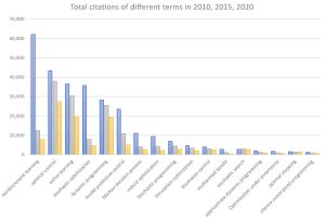 The graph to the right shows the growth over the years 2010, 2015 and 2020 in the citations of major terms associated with sequential decisions (usually under uncertainty). “Reinforcement learning” stands out not just for its popularity, but its dramatic growth from 2015 to 2020 (“stochastic optimization” is also growing quickly, perhaps helping to emphasize the importance of handling uncertainty).
Not surprisingly, the scope of problems has expanded far beyond the problems familiar to the original core community. Even articles that attempt to communicate the breadth of applications (an example is here) do not come close to capturing all of the problems that are being addressed under the umbrella of “reinforcement learning.” And not surprising, this breadth of problems is pushing the boundaries of methodology. Just as the methods of reinforcement learning grew from the original focus on Q-learning to the much wider range of methods in the second edition of Sutton and Barto’s Reinforcement Learning, the field, as we speak, is growing into new application domains, sparking a continuing growth in the library of methods for solving these problems.
It is specifically the massive popularity of “reinforcement learning” that forces us to ask the question: what does it mean? The challenge of defining the term can be attributed to the vast diversity of problems that fall within the framework of RL problems. It should not be surprising that we are not going to be able to solve the universe of RL problems with a single method, opening up the question: just what are RL problems, and what are RL methods?
Perspectives of reinforcement learning
What is meant by the term “reinforcement learning” has been evolving over the years (the same evolution has been happening in sister communities under the broad heading of “stochastic optimization”). Below I use three of the most popular sources: Rich Sutton and Andy Barto (who introduced the term), Ben van Roy (an early pioneer and well-known RL researcher), and Dimitri Bertsekas, widely known for his books on dynamic programming and optimal control (also neuro-dynamic programming, approximate dynamic programming, as well as reinforcement learning). Finally, while there are many resources on the internet (such as this page), I have also included the Wikipedia page on reinforcement learning. I then contrast these perspectives with the approach used in my new book, and close with some comments on the evolution of “reinforcement learning.”
Rich Sutton and Andy Barto (S&B) – 2018 edition of Reinforcement Learning: An introduction
In the 2018 edition of Reinforcement Learning: An introduction, S&B note [p. 2] “Reinforcement learning… is simultaneously a problem, a class of solution methods that work well on the problem, and the field that studies this problem and its solution methods.” I particularly like the comment that follows: “It is convenient to use a single name for all three things, but at the same time [it is] essential to keep the three conceptually separate. In particular, the distinction between problems and solution methods is very important in reinforcement learning; failing to make this distinction is the source of many confusions.” (I strongly agree with this, as you will see below.)
In the following paragraph they add: “Markov decision processes are intended to include just these three aspects – sensation, action, and goal – in their simplest possible forms without trivializing any of them. Any method that is well suited to solving such problems we consider to be a reinforcement learning method.” Below I will raise the question of whether a method for solving (approximately) an MDP, but which does not involve any learning (these include methods known as “model predictive control”), constitutes a reinforcement learning method.
On p. 6, S&B go on to say “… one can identify four main subelements of a reinforcement learning system: a policy, a reward signal, a value function and, optimally, a model of the environment.” This is where S&B and I part ways. S&B seem to define value functions as fundamental to a reinforcement learning “system,” but this is part of a method for solving RL problems. Further, value functions are fundamental to only one of four classes of methods (policies) – see “Designing policies” below. A core challenge of an RL problem is designing a method to solve the problem, and it is easy to find examples of policies within their own book that do not involve value functions. For example, parameterized policies that are optimized by their policy gradient method, or parameterized UCB policies for bandit problems – neither of these policies use value functions.
Ben van Roy (professor, Stanford University)
At a “reinforcement learning and optimal control” workshop in 2018 (organized by people in optimal control), Ben van Roy (a renowned RL researcher at Stanford, and early pioneer of the field) described reinforcement learning as:
- A problem class consisting of an agent acting on an environment receiving a reward.
- A community that identifies its work as “reinforcement learning.”
- The set of methods developed by the community using the methods it self-identifies as “reinforcement learning” applied to the problem class.
This description effectively describes “reinforcement learning” as any method used by the reinforcement learning community for solving problems that can be described as an agent acting on the environment receiving a reward. The community used to be a fairly well defined set of researchers in computer science, but as the visibility of the field grew (through successes solving games such as chess and Go), so did the breadth of the communities identifying themselves with reinforcement learning.
Ben’s characterization of reinforcement learning effectively says that it is whatever the “RL community” is doing to solve a problem that involves “an agent acting on an environment receiving a reward.” I like the style of defining “reinforcement learning” by how it is used in the community as opposed to some abstract notion (this is how Webster defines words). But we have to be aware that as I outlined above, the scope of problems that fall under this general description is huge and growing quickly.
I have two issues with Ben’s characterization of “an agent acting on the environment receiving a reward:”
- First, we have to define what it means to “act on the environment.” Is observing the environment an instance of “acting on the environment”? If someone pulls out a pair of binoculars to observe what types of birds are in an area, is that “acting on an environment”?
- Second, what if our “agent” has only one action to choose from, so she is always making the same action. I am quite sure that no-one would view that as a reinforcement learning problem. Implicit in the idea of “acting on the environment” is the idea that there is a choice of actions. In other words, the agent needs to make a decision.
Below, I am going to replace Ben’s “agent acting on an environment and receiving a reward” with “sequential decision problem” which might be viewed as equivalent, or more general (depending on how you interpret Ben’s problem definition).
Dimitri Bertsekas – Reinforcement Learning and Optimal Control (2019) (and Dynamic Programming and Optimal Control: Approximate Dynamic Programming (2012))
In his recent book Reinforcement Learning and Optimal Control (RLOC), Bertsekas states in his preface [page ix] “In this book we consider large and challenging multistage decision problems, which can be solved in principle by dynamic programming (DP for short), but their exact solution is computationally intractable. We discuss solution methods that rely on approximations to produce suboptimal policies with adequate performance. These methods are collectively known by several essentially equivalent names: reinforcement learning, approximate dynamic programming, and neuro-dynamic programming. We will use primarily the most popular name: reinforcement learning.” I think most readers would equate these terms with methods based on approximating value functions, but the book is much broader than this, raising the question of whether “reinforcement learning” actually is equivalent to these other terms.
RLOC mentions policies such as upper confidence bounding, but does not recognize that the tunable parameter(s) used in all UCB policies have to be tuned, which is its own optimization problem. The book mentions model predictive control (MPC), but, as is typical, only discusses the version that uses a deterministic lookahead (many people equate “MPC” with deterministic lookahead models). It also includes a brief mention of Monte Carlo tree search which is typically used as a (possibly stochastic) lookahead policy, although RLOC does not present MCTS, MPC, policies based on value function approximations and parameterized policies as competing approaches to solve the same problem.
The terms “approximate dynamic programming” and in particular “neuro-dynamic programming” (a term introduced in 1996 in the monograph Neurodynamic Programming by Bertsekas and Tsitsiklis) focus on solving sequential decision problems using approximations of Bellman’s equation, which means some form of value function approximation. However, the idea of a parameterized function for the policy (which does not use a value function approximation) has been a persistent presence through the years. In his RLOC book (2019), Bertsekas explicitly includes “approximation in policy space” (which might include some form of parameterized policy) as falling within the broad umbrella of reinforcement learning. I think this hints at the evolution of how all of us are thinking about the field.
Wikipedia
There are a large number of “RL” tutorials on the internet. I am going to use the one on Wikipedia since this is probably the most visible.
Wikipedia starts by stating: “Reinforcement learning (RL) is an area of machine learning concerned with how intelligent agents ought to take actions in an environment in order to maximize the notion of cumulative reward.” [Side note: you can optimize either cumulative or final reward – both are quite relevant to the RL literature.] It then makes a widely repeated claim: “Reinforcement learning is one of three basic machine learning paradigms, alongside supervised learning and unsupervised learning.” This would indicate that a policy (such as model predictive control) that does not involve learning is not a form of “reinforcement learning” even though it is a method for solving a sequential decision problem.
Wikipedia states the problem of finding the best policy, and identifies two approaches for creating policies: value function estimation and direct policy search (as found in Bertsekas’ RLOC). This list seems to ignore direct lookahead policies (my name), also known as “model predictive control” (an important example is Monte Carlo tree search). Nor does it mention upper confidence bounding for pure learning problems.
Warren Powell – Reinforcement Learning and Stochastic Optimization (2022)
I took a different approach in my new book (which builds on my book Approximate Dynamic Programming: Solving the curses of dimensionality (2011)) by first dividing problems into two broad classes: pure learning problems (these are settings where the problem does not depend on the state variable, just the beliefs about the problem), and general state-dependent problems (where the problem is evolving through a combination of exogenous inputs and/or endogenous decisions). Then, for both classes, I adopt a general five-element modeling framework (summarized below) that describes any sequential decision problem (using any of a number of objective functions). This framework involves optimizing over policies, where I identify four (meta) classes of policies that include any method for making decisions (also summarized below).
RLSO is the first book to approach reinforcement learning from the perspective of a universal modeling framework (closely modeled after that used in the optimal control literature) and the first to identify the four classes of policies. Chapter 11 (downloadable from RLSO) describes all four classes, along with a number of hybrids that cut across different classes. Unresolved, however, is whether this might be a modern interpretation of reinforcement learning, or if reinforcement learning is a subset of this broader framework.
A better title for my book would have been “Sequential Decision Analytics” which introduces a phrase no-one has ever heard of, and which ignores the overlap with reinforcement learning as well as stochastic optimization (and optimal control, as well as a dozen other fields). My book covers four classes of policy gradient algorithms (chapter 11), introduces the idea of parameterizing deterministic optimization models (called cost function approximations, chapter 13), and of course includes policies based on lookahead approximations, spanning both value function approximations (whose coverage spans chapters 14-18) and direct lookahead models (chapter 19). Chapter 19 provides a general presentation of both deterministic and stochastic lookahead models, including both parameterized deterministic lookaheads, as well as a wide range of approximations for stochastic lookahead models.
Some observations:
Sutton and Barto introduced the phrase “reinforcement learning” in the context of approximation algorithms for dynamic programs (the term dates to the early 1900s in the psychology literature), and as of this writing have the only book called “Reinforcement Learning.” While it would be reasonable to refer to this book as the bible of reinforcement learning, it seems clear that S&B still seem to equate “reinforcement learning” with methods based on approximating value functions.
I like Ben’s approach of describing “reinforcement learning” based on how the term is used, rather than any formal definition. In a community as large as the RL community has grown to, this is the only practical strategy. However, I also endorse the comment made by S&B: “It is convenient to use a single name for all three things, but at the same time essential to keep the three conceptually separate.”
The term “reinforcement learning” has evolved from the original focus on approximating value functions to a broader set of strategies. Both Bertsekas (in RLOC) and I (in RLSO) outline a set of algorithms that is broader than what can be found in Sutton and Barto’s RL book, but it is important to note that even S&B’s Reinforcement Learning covers a wide range of algorithms than can be found in their first edition.
I think it is fair to say that the meaning of “reinforcement learning” is growing, but it is hard to say right now (or, I think, at any point in time) precisely what the term refers to. Both Dimitri and I chose to title our books “Reinforcement Learning and …” where Dimitri uses “and Optimal Control” (reflecting his background in control theory) while I use “and Stochastic Optimization” (reflecting my background in operations research). For example, both RLOC and RLSO include deterministic lookahead policies (often referred to as model predictive control or MPC), which is a popular method for solving certain classes of sequential decision problems, but MPC generally does not involve any learning. Will “reinforcement learning” grow to include MPC, or will there be boundaries that limit the scope of “reinforcement learning” as a field that addresses sequential decision problems?
Following S&B, I think it is particularly important today to maintain the distinction between RL problems and RL methods. Rather than trying to define either of these based on how these terms are used in the community today (I have no idea how to do this), I am going to look at how the field is evolving, and then project where the field is going to end up:
- RL problems – Every RL problem is a sequential decision problem, so I am going to starting by referring to the problem class as sequential decision problems (I describe this problem class formally below). As of this writing, I cannot say that every sequential decision problem is an RL problem, but this may change.
- RL methods – Every RL method for making decisions is a form of policy. Below I argue that there are four classes of policies, and I further claim that these four classes include every method that has ever been suggested in the research literature or used in practice (including methods that have not even been invented yet). This means every RL method falls in these four classes of policies, but not every method within these four classes involves learning, so it is not yet clear that they will be viewed as “reinforcement learning.”
I provide a more detailed description of sequential decision problems and the four classes of policies below.
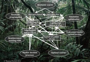
This characterization of problems and methods reflects an evolution that is taking place in other communities working in this space (dynamic programming, optimal control, stochastic optimization, simulation optimization, stochastic programming, multiarmed bandit problems, …) that are going through the same growth in terms of the scope of problems and variety of methods (this is illustrated in the graph to the left). Today, the overlap between these communities is significant and growing, so much so that even these other communities are starting to describe their work as “reinforcement learning.” The snowball effect cannot be ignored.
Ultimately, I think it will be more appropriate to adopt a broader name for a field. I suggest “sequential decision analytics” and make an effort at outlining the dimensions of this field here. However, guessing at how languages will evolve in a community as large as this is an exercise in futility (just look at all the different names associated with approximating value functions before “reinforcement learning” emerged).
Below I provide a brief introduction to modeling sequential decision problems (which requires optimizing over policies), and then designing policies. As I watch the evolution of the work taking place under “reinforcement learning,” my belief is that eventually the RL community will have to recognize the space of sequential decision problems (some might say that this has already happened), and all four classes of policies (this requires more time).
Sequential decision problems
Sequential decision problems describe any setting where we intermingle making decisions and then making observations that affect the performance of the decision. Any sequential decision problem can be written as the sequence
state, decision, information, state, decision, information, …
or using notation (S being state, x being decision, and W being new information):
(S^0,x^0,W^1,S^1,x^1,\ldots,S^n,x^n,W^{n+1},X^{n+1},\ldots,S^N)
We are indexing “time” using an iteration counter n, but we could use time t, in which case we would write the state as S_t, decision x_t, and exogenous information W_{t+1}.
Each time we make a decision we receive a contribution C(S^n,x^n). We make decisions x^n with a function (called a policy) X^\pi(S^n). For these problems, the decisions x^n could be binary, discrete or continuous, scalar or vector-valued.
The goal is to find the best policy where we might optimize the objective function
\max_\pi \mathbb{E} \left\{\sum_{n=0}^N C(S^n,X^\pi(S^n))|S^0\right\}.
There are variations of this objective function; here we are maximizing the cumulative reward, but we might also maximize the final reward after a series of learning iterations. We can also use risk measures instead of expectations.
There are five components of any sequential decision problem:
- The state variable S^n that contains whatever we know (or belief) after n observations.
- The decision x^n which is made using a (yet to be designed Policy X^\pi(S^n).
- The exogenous information (not present in all problems) W^{n+1} that is the information that arrives after we choose x^n.
- The transition function which describes how the state variables S^n given the decision x^n and exogenous information W^{n+1}. I like to write this as
S^{n+1}=S^M(S^n,x^n,W^{n+1})
- The objective function
Recognizing that objective functions can come in different styles, I claim that these five components describe any sequential decision problem. Note that this modeling framework is actually well established in the optimal control community, but it nicely describes the sequential decision problems found in reinforcement learning.
A key feature of this canonical framework is searching over policies (which are forms of functions). This is comparable to the challenge faced in machine learning where the search is for the best statistical model (which is also a function). The most common mistake is to assume that the starting point for designing policies is Bellman’s equation. This is simply not true. In the next section I describe the four classes of policies that spans every method for making decisions.
Designing policies
The core challenge of sequential decision problems is the design of policies (modeling uncertainty is also a nice challenge). There are two broad classes for designing policies:
- The policy search class – These are policies that have to be tuned over time to work well in terms of the performance metric (maximizing rewards, minimizing costs, …). This tuning is usually done offline in a simulator, but may be done in the field.
- The lookahead class – These policies work by finding the action now, given the state we are in, that maximizes the one-period reward plus an approximation of the downstream value of the state that the action takes us to (this may be random).
Each of these classes are divided into two additional subclasses. The policy search class includes:
- Policy function approximations (PFAs) – This is the simplest class, and includes analytical functions that map state to action. These include lookup tables (if patient is male, smoker, overweight then describe this drug), , parametric models (buy-low, sell-high policies in finance, order-up-to inventory policies, neural networks), and nonparametric models (such as locally linear models).
- Cost function approximations (CFAs) – These are parametrically modified optimization problems. For example, let \mu_x be the reduction in blood sugar from drug x, and let \bar{\mu}_x be our estimate of the reduction for a new patient. We could just choose the drug that maximizes \bar{\mu}_x, but we have a lot of uncertainty. Let \bar{\sigma}_x be the standard deviation of this estimate. A good policy for choosing a drug to test would be given by x=\argmax_x\left(\bar{\mu}_x + \theta \bar{\sigma}_x\right), where \theta is a tunable parameter. Increasing \theta encourages trying drugs where there is more uncertainty. Parametric CFAs are widely used in practice, since they can be any deterministic optimization problem where tunable parameters have been introduced to handle uncertainty. For a detailed introduction to parametric CFAs, click here.
The lookahead class can also be divided into two subclasses:
- Policies based on value function approximations (VFAs) – If we are in a state (this might capture how much inventory we have on hand, the state of a game, the location and velocity of a robot), and take an action (e.g. ordering more inventory, making a move, applying forces) that takes us to a new state, we might estimate the value of being in this new state. This estimate (we can rarely do this exactly) is known as a value function approximation. VFAs are comparable to the Q-factors in Q-learning, and can be approximated using any of the tools from machine learning.
- Direct lookaheads (DLAs) – The easiest example of a DLA is a navigation system that decides whether you should turn or go straight by finding the best path (or at least an approximation) to the destination. This path can be updated periodically during the trip. Another example of a DLA is when you plan several moves into the future when playing a game to determine what move you make now.
Here is my major claim: These four classes of policies (PFAs, CFAs, VFAs and DLAs) cover every possible method for making decisions over time that has been used by any of the research communities working on sequential decisions, along with any method used in practice. In other words, I claim that these four classes are universal, which means they include whatever you might be using now (without knowing it).
This is a major point of departure from the other books on reinforcement learning, which have started to describe an ever-broadening library of methods, without recognizing that each method belongs to one of these four classes of policies.
My most complete description of the four classes of policies (including a number of hybrids formed of policies from two, three or even all four classes) is Chapter 11 of my new book Reinforcement Learning and Stochastic Optimization. Chapter 11 can be downloaded from the RLSO webpage.