Reinforcement learning versus sequential decision analytics

Warren B Powell
Professor Emeritus, Princeton University

I have been working on stochastic optimization problems (more specifically, sequential decision problems) since 1981 when I started at Princeton, originally motivated by the challenge of optimizing fleets of trucks for the truckload trucking industry (simplistically you can think of this as Uber for freight).  My career would have me working on virtually every mode of freight transportation, along with the optimization of energy systems, health (public health and medical decisions), finance, e-commerce and optimal learning in materials science.

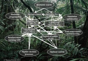
I followed the early work in reinforcement learning which developed under the name of approximate dynamic programming in fields such as engineering and operations research. My path through a wide range of problems also exposed me to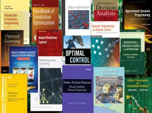 the work in a number of fields that were identified by names such as dynamic programming, Markov decision processes, stochastic programming, simulation optimization, robust optimization, stochastic search, optimal control (including variants such as model predictive control), along with the multiarmed bandit problems and optimal learning.  I started to call these disparate communities the “jungle of stochastic optimization.” 

My background produced my latest book, Reinforcement Learning and Stochastic Optimization: A unified framework for sequential decisions. The book covers most of the classical material contained in Sutton and Barto’s Reinforcement Learning: An introduction, but the styles of the two books are quite different.   

I designed this webpage to explore the differences between the two books, and share my thoughts on the evolution of the field of reinforcement learning and its relationship to other communities working on sequential decision problems.  Given the rapid evolution, I found that there is significant confusion about precisely what is meant by “reinforcement learning,” a topic I cover on my “What is RL” webpage.

The discussion is divided into the following topics (this is a developing webpage):

• Topic 1: The evolution of the field of reinforcement learning – From Sutton and Barto (1994), to Sutton and Barto (2018), to… the universal framework?
• Topic 2: Differences between Sutton and Barto’s Reinforcement Learning: An introduction and my Reinforcement Learning and Stochastic Optimization: A universal framework for sequential decisions
• Topic 3: From Q-learning to the four classes of policies
• Topic 4: Which policies are most popular? It is not what you will expect
• Topic 5: Choosing notation – Notation matters, and here I explain what is wrong with the standard notation of RL, and why I made my choices

Topic 1: The evolution of the field of reinforcement learning – From Sutton and Barto (1994), to Sutton and Barto (2018), to… the universal framework?

The field of reinforcement learning is undergoing rapid evolution, as have the other fields that deal with sequential decision problems.  In 1998, the first edition of Sutton and Barto’s Reinforcement Learning: An introduction appeared, focusing almost entirely on algorithms for approximating value functions.

In 2018, Sutton and Barto published the second edition of their book.  This time, it covered a variety of algorithms, raising the question: just what is “reinforcement learning”?  Is it a method? or a problem? 

In the 2018 edition of Reinforcement Learning: An introduction, S&B note [p. 2] “Reinforcement learning… is simultaneously a problem, a class of solution methods that work well on the problem, and the field that studies this problem and its solution methods.” (Click here for a more complete discussion of the question “What is RL.”)

The field of reinforcement learning is undergoing the same evolution as most of the other major fields that work on sequential decision problems.  As the community grows, it addresses a wider range of problems.  Inevitably, no single method works on all problems, so people create new methods.  What is unusual about the RL community is that, as they introduce new methods, they keep calling everything “reinforcement learning.”

My approach: First recognize that the common thread among all of these problems is that they are some form of sequential decision problem.  Second, I found that every single method introduced for making decisions falls in one of the four classes of policies, or a hybrid.  I discuss the four classes of policies, and hybrids, in depth in chapter 11 of RLSO (this can be downloaded from the RLSO webpage here).

Although my book (RLSO) covers a wide range of methods, it clearly identifies the problem class as sequential decision problems which can be modeled  using the universal framework.  It then introduces the four classes of policies (plus hybrids) which includes not only every method for making decisions that has been introduced in the literature (or used in practice), it also includes methods that haven’t even been invented yet (these are meta-classes).  See Topic 3 (below) for a brief discussion of the four classes of policies.

For this reason, I view my book as the natural endpoint for reinforcement learning, as well as all the other fields that deal with decisions under uncertainty (I represent these with “stochastic optimization”).  

Topic 2: Differences between Sutton and Barto’s Reinforcement Learning: An introduction (RL) and my Reinforcement Learning and Stochastic Optimization: A universal framework for sequential decisions (RLSO)

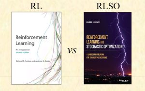
It is time to clarify the differences between “reinforcement learning” (as represented by Sutton and Barto’s Reinforcement Learning: An introduction) and the emerging field of sequential decision analytics, as captured by my book Reinforcement Learning and Stochastic Optimization: A unified framework for sequential decisions.  Below, I use “RL” to refer to Sutton and Barto’s “Reinforcement Learning” and “RLSO” to refer to my “Reinforcement Learning and Stochastic Optimization.”  For more on RLSO, click here. 

• RLSO presents a universal framework for any sequential decision problem, where:  

• • Every RL problem is a sequential decision problem (RL is used for solving “Markov decision problems” – just another word for “sequential decision problem.”).  See chapter 9 of RLSO.
  • Every RL algorithm is a sequential decision problem (see chapters 5 and 7 of RLSO). 
  • RLSO describes the modeling frameworks for each of 15 different fields that address sequential decision problems, using the notation of that field (see section 2.1).

• Every method for solving an RL problem falls in one of the four classes of policies in the universal framework for sequential decision problems. See chapter 11 of RLSO (downloadable from the RLSO webpage).  You can find examples of policies from each of the four classes of policies in RL: 
  • The “policy gradient method” is used to tune the parameters of PFAs (see chapter 12 of RLSO).
  • Upper confidence bounding is a type of CFA (cost function approximation – see https://tinyurl.com/cfapolicy and chapter 13 of RLSO).
  • All policies based on Q-learning (etc) are forms of VFAs (these are covered in chapters 14-18 in RLSO).
  • Monte Carlo tree search is a form of DLA (direct lookahead approximation). MCTS along with a wide range of direct lookahead approximations are covered in chapter 19.
• Every multiarmed bandit problem is a form of derivative-free stochastic search, and vice versa.  These are sequential decision problems that have been solved using each of the four classes of policies.  These are all covered in chapter 7.
• Parameter tuning can be solved using either derivative-based or derivative-free stochastic search.  Chapter 5 is dedicated to derivative-based stochastic search (including SPSA – simultaneous perturbation stochastic approximation – which is useful for multidimensional parameter vectors).  Chapter 6 is the first chapter dedicated to the rich topic of stepsizes.
• RL covers only the “policy gradient theorem” which is a type of derivative-based stochastic search.  RLSO (in chapter 12) covers four different strategies for derivative-based stochastic search:
  • Derivative-based stochastic search using exact derivatives for problems with continuous states and controls.
  • Derivative-based stochastic search using exact derivatives for discrete actions (the “policy gradient theorem”).
  • Numerical derivatives (this is much simpler than the first two).
  • Derivative-free stochastic search (using any of the methods from chapter 7).
• RLSO has five chapters dedicated to methods based on approximating value functions:
  • Chapter 14 is on exact dynamic programming, and reviews both discrete dynamic programs as well as special cases of continuous dynamic programs, including the well-known “linear-quadratic regulation” known in control theory.
  • Chapter 15 is on backward ADP for finite-horizon problems.
  • Chapters 16 and 17 represent classical material on ADP, including temporal-difference learning and Sutton’s projected Bellman operator for linear VFAs.
  • Chapter 18 focuses on the types of dynamic programs that arise in multiperiod resource allocation problems.  These are high dimensional, but enjoy the property of concavity of the value function, making possible the use of specialized methods such as Benders decomposition (widely known as “stochastic dual dynamic programming” or SDDP).
• RL includes a brief description of Monte Carlo tree search, which is a special class of lookahead policy (solved on a rolling basis).  RLSO (chapter 19) includes the most complete discussion of lookahead policies available anywhere:
  • Section 19.1 introduces the notation for an approximate lookahead model, and establishes the relationship between the lookahead model (which we solve to make a decision) and the base model, which is where we evaluate the policy.
  • Sections 19.2 describes six different strategies for creating a lookahead model.
  • Section 19.3 shows how to introduce risk in the lookahead model.
  • Section 19.6 introduces deterministic lookahead models, and describes the powerful idea of using parameterizations (this creates a hybrid DLA/CFA policy).
  • Section 19.7 describes stochastic lookahead policies, and shows how any of the four classes of policies can be used for the “policy-within-a-policy.” 
  • Section 19.8 describes classical (pessimistic) MCTS in detail, and then introduces (for the first time in a book) optimistic MCTS, which optimally solves a sampled future within the search tree, producing an optimistic estimate of the future.
  • Section 19.9 describes the concept of scenario trees used in the stochastic programming literature for problems where decisions are vector-valued (this was first introduced in the 1950s by George Dantzig).  

For more on the general field of sequential decision analytics, click here for a web page of links to different resources.

Topic 3: From Q-learning to the four classes of policies

The field of reinforcement learning followed my own early path: I started with a particular type of resource allocation problem (managing fleets of vehicles) where Bellman’s equation seemed to be a natural strategy.  Deciding to send a vehicle from region i to region j required understanding the value of being in region j.  The challenge with my setting was that I did not have a single vehicle: I needed to manage fleets of hundreds, even thousands, of vehicles.  The state space exploded, which meant that I needed to approximate the downstream value.  

As my range of applications expanded, the techniques that I found myself using also grew.  This paralleled the path followed in reinforcement learning, as well as other communities such as stochastic search, optimal control, and simulation optimization.

I came to realize that all of these fields were steadily discovering methods for making decisions that fell into four classes:

1. Policy function approximations (PFAs) – These are analytical functions that determine a decision given an analytical function of the information in the state variable.  Examples include: order-up-to policies for inventory problems, buy-low, sell-high policies in finance, linear decision rules, Boltzman policies.
2. Cost functions approximations (CFAs) – These are parameterized versions of simplified optimization problems.  Examples include upper confidence bounding, parameterized linear programs, modified shortest path problems.
3. Value function approximations (VFAs) – This covers the entire class of policies that depend on an approximation of a value function (often equated with “reinforcement learning”).
4. Direct lookahead approximations (DLAs) – Here we optimize over some typically approximate version of the problem over some horizon to determine what to do now.  I like to divide this class into two subclasses:
   1. Deterministic lookaheads (which might be parameterized) – This is often what people mean when they say “model predictive control.” 
   2. Stochastic lookaheads – In chapter 19, section 19.7, I provide a variety of strategies for approximating stochastic lookaheads, focusing on the problem of designing policies within the lookahead model.

All of these policies are represented in Sutton and Barto’s Reinforcement Learning:

• PFAs are parameterized policies that would be optimized using the “policy gradient theorem” in S&B.  Note that the policy gradient theorem is not a policy; it is a method for tuning a parameterized policy for certain types of policies (e.g. Boltzman) and problems (discrete states and actions).
• A nice example of a CFA is any form of upper confidence bounding for multiarmed bandit problems.
• VFAs represent the entire class of methods based on approximating value functions.
• Monte Carlo tree search, which can be used for both deterministic as well as stochastic problems, are a form of direct lookahead. 

The graphic below illustrates the adoption of each of the eight most important fields of the four classes of policies (wider lines means earlier adoption).

Topic 4: Which policies are most popular?

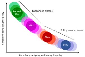I am constantly being asked: how to choose which class of policy to use? The figure to the right illustrates the tradeoff between the complexity in designing and tuning a policy (I assume this is for nontrivial applications) versus the complexity in computing a policy.  For example, if we want to try to create a parametric policy, designing it for a complex problem can be quite hard to do, although it will be easy to compute if we are successful.  By contrast, a stochastic direct lookahead can be hard to compute, but creating the policy is relatively brute force – we just have to create a forward simulator of our problem.

See chapter 11, section 11.10, for my discussion of how to choose among the four classes of policies (this is downloadable from RLSO).  

The academic literature has been heavily biased first toward policies based on approximating Bellman’s equation, and second toward policies based on some form of stochastic lookahead (think of Monte Carlo tree search or stochastic programming).  However, in practice I have found that the five types of policies can be organized into three categories, sorted from the ones that are most widely used to the policies that are least used:

Category 1: The most popular policies consist of:

• • Policy function approximations (PFAs) – These are the simplest policies, designed for the simplest problems (and most decision problems are simple).
  • Cost function approximations (CFAs) – These are parameterizations of simple optimization problems (the optimization problem may be a simple sort, or simple linear programs).
  • Deterministic direct lookahead approximations (deterministic DLAs) – Think of google maps, which solves a deterministic approximation of the future to determine what direction to move now.

Category 2: Stochastic direct lookaheads – Sometimes we need a lookahead, but we need to recognize that the future is uncertain.

Category 3: Policies based on value function approximations (VFAs) – After decades of focusing on approximate dynamic programming (and writing a major book on the topic), I am now convinced that policies based on approximate dynamic programming are the most difficult to use, and will be the least-used policy in practice.

Within category 1, the choice of which of the three policies to use will typically be obvious from the application.  In the universe of decision problems that we encounter across the vast range of human activities, I am now convinced that policies in category 1 will be used the vast majority of the time (hint: this is what is happening now).  However, often overlooked is that the policies in category 1 depend on tunable parameters, and as I say in RLSO: tuning is hard! See my discussion of parameter tuning in chapter 12 of RLSO (section 12.4 discusses the most popular strategies).

Note that in my opinion, based on many years of research focused specifically on policies based on approximating Bellman’s equation, I became convinced that while this is a very powerful strategy, it is useful for just a narrow set of applications.  As an indication: in the universe of problems that require making decisions, real applications of Bellman’s equation are quite rare (one good example of the use of approximate dynamic programming is the software at my company, Optimal Dynamics, that uses VFAs to optimize the assignment of drivers over time).  

Topic 5: Choosing notation – Notation matters, and here I explain my particular choices.

I spent decades working out my notational system.  in section 2.1 of RLSO, I present 15 different fields using the notation most popular in that field.  My framework is closest to that used in optimal control, but with different notation.  Specifically:

• I use S_t for the state at time t (if we are using time), or S^n for the state after n experiments (n may count iterations, observations, experiments, or arrivals of customers).  I use S_t for the state at time t which is a random variable.  If I just want a particular state, I would use s.  Some notes:
  • The Markov decision process field, which was adopted by reinforcement learning, uses s without any time index.
  • The optimal control community uses x_t for the state at time t  which conflicts with the entire field of math programming which uses x_t for decision.
• The initial state S_0 contains the initial values of any variables that change over time, as well as any parameters that do not change at all.
• I use x_t for decisions, where x_t may be binary, a member of a discrete set, a continuous scalar, or continuous/discrete vectors.  In other words, anything. Notes:
  • The RL/Markov decision process community uses a for action, which is almost always discrete.
  • The optimal control community uses u_t, where it is most common for x_t to be a continuous, low-dimensional vector (such as the force applied in each direction).
• I use W_{t+1} for the exogenous information that first becomes known at time t.  Said differently, it is the information that arrives after decision x_t is made, but before decision x_{t+1} is made.  Notes:
  • The only field that seems to have standard notation for the exogenous information process is optimal control, which uses w_t for the information that arrives between t and t+1.  This means that w_t is random at time t, which can cause serious confusion when modeling complex stochastic systems. 
  • I use the convention that any variable indexed by t is known at time t (if using a counter n, it means that any variable indexed by n depends on observations W^1, \ldots, W^n.
• The optimal control community uses x_{t+1} = f(x_t,u_t,w_t) to model the transition function.  With my notation, I use S_{t+1} = S^M(S_t,x_t,W_{t+1}).  Notes:
  • I love the concept of a transition function (used widely in engineering by the optimal control community, but is not standard in operations research or computer science.
  • But, “f” for function is notation that has many uses.  To avoid taking up such valuable real-estate in the alphabet, I went with S^M(\cdot) which stands for “state transition model.”  
  • Note how the equation S_{t+1} = S^M(S_t,x_t,W_{t+1}) nicely communicates that we are taking the state S_t which is known at time t, the decision x_t which is determined from x_t=X^\pi(S_t) (which means it is known at time t).  It also communicates that W_{t+1} is not known at time t, but it is known by time t+1 so we can compute the next state S_{t+1}.