From reinforcement learning to sequential decision analytics

Warren B Powell

“Reinforcement learning” has been undergoing an evolution from the early work in the 1980s-1990s where it focused on a form of approximate dynamic programming called Q-learning, to the study of a diverse range of algorithmic strategies for sequential decision problems.  Since this time it has continued to evolve, along with a number of other communities that also work on sequential decision problems.  I feel I have anticipated where those entire evolution is likely to end up.

Please enter any comments on the ideas in this page at https://tinyurl.com/RLSOcomments.

My new book, Reinforcement Learning and Stochastic Optimization: A unified framework for sequential decisions (RLSO) is the first book to propose a universal framework that models any sequential decision problem, from pure learning (multiarmed bandit) to complex resource allocation problems.  We formally pose the problem of optimizing over policies (methods for making decisions), and present four classes of policies that include any method for making decisions.  The entire book is organized around this universal modeling framework and the four classes of policies.

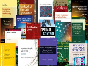This modeling framework spans 15 distinct communities that work on sequential decision problems. These communities use eight distinct notational systems, and feature a wide range of solution techniques tailored to specific problem domains that arise in different fields.  However, there are four fields that make particularly important contributions: Markov decision processes, math programming, optimal (stochastic) control, and stochastic search (derivative-based and derivative-free).  Of course, we will draw heavily on the tools of machine learning and Monte Carlo simulation.

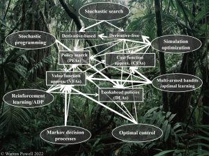Most of these communities have been evolving from an initial algorithmic strategy to different strategies that span the four classes of policies.  This evolution has been taking place in a number of communities that work on sequential decision problems – the best illustration is the second edition of Sutton and Barto’s Reinforcement Learning book that now includes policy gradient methods, upper confidence bounding and Monte Carlo tree search.  In the graphic to the right, I have listed seven of the most prominent communities: stochastic search (derivative-free and derivative-based), simulation optimization, multiarmed bandits, optimal control, Markov decision processes, reinforcement learning and stochastic programming.  I then show which of the four classes of policies are actively studied in each community (wider lines represent the policies that were initially studied).

Below I list the differences between how these problems are described and solved in the reinforcement learning literature, and the modeling and solution approach that I use in RLSO.  I claim that my approach better represents how people in the RL community actually write their software, and the algorithms that are actually being used (including algorithms that have not yet been adopted!). Below I touch on three issues:

• Modeling – This addresses notational choices and the elements of a sequential decision problem.
• Designing policies – I identify four (meta)classes of policies that include any method for making decisions in a sequential decision problem.
• Policy search/parameter tuning – I have been surprised at how often the RL community ignores the important step of tuning parameters within a policy.

Modeling

•  The modeling framework. Reinforcement learning adopted the modeling framework of Markov decision processes, which captures state spaces, action spaces, the one-step probability transition matrix P(s'|s,a) which is the probability of transitioning from state s to state s’ after taking action a, and the reward r(s,a). This framework was designed by mathematicians, and offers virtually no value in terms of modeling real problems. I draw heavily from the modeling framework used in optimal control (but not the notation), where I can model any sequential decision problem using five components:
  • State variables S_t giving all the information at time t to model the system from time t onward.  We could use S^n to model the information after n observations/iterations/experiments.  State variables are widely misunderstood (neither Sutton and Barto nor Bertsekas define a state variable).  See chapter 9, section 9.4 of RLSO for a detailed definition and discussion of state variables.
  • Decision variables x_t – While the RL community tends to focus on discrete actions a, x_t (adopted from the field of math programming, used around the world) can be binary, discrete, continuous, and vectors of continuous and/or discrete variables (in other words, anything).  Decisions at time t have to reflect any constraints x_t \in X_t.  We make decisions using a method we call a policy, that we represent using X^\pi(S_t), but we defer designing policies until later (this is the basis of what I call “model first, then solve”).
  • Exogenous information W_{t+1} – This is the information that arrives between t and t+1 (or we can use W^{n+1} is what we observe in the n+1st experiment).  Exogenous information can come from Monte Carlo simulation using a probability distribution, or it can come from historical data or field observations (in an online setting). 
  • Transition function S_{t+1}=S^M(S_t,x_t,W_{t+1}) – Transition functions are widely used in optimal control and engineering, where they use x_{k+1}=f(x_k,u_k,w_k) to represent the transition function from state x_k at ”time” k, apply control u_k, and then observe w_k (which is random at ”time” k).  Our notation S^M(\cdot) stands for ”state transition model” (or ”system model”).  The one-step transition matrix used in the RL/MDP communities is almost never computable, while transition functions are easy to compute.  When people talk about ”simulating the transition matrix” they actually mean using the transition function.
  • The objective function – We prefer to maximize contributions C(S_t,x_t) (or minimize costs).  Our objective function optimizes over policies X^\pi(S_t).  Objective functions come in different flavors: final reward/cumulative reward, expectation/risk/ … If we use a classical expectation-based objective of a cumulative reward, we would write:

\max_{\pi} \mathbb{E} \left\{\sum_{t=0}^T C(S_t,X^\pi(S_t))|S_0 \right\}

•  From model to software.  There is a one-to-one relationship between the modeling framework I use and the software implementation.  Anyone who writes a simulation model of a sequential decision problem can directly translate their code back to the modeling framework above.  This is true of anyone working in reinforcement learning using the standard modeling style in this community, even if they are not familiar with the modeling framework in RLSO.
•  Finite-horizon vs. steady state.  For historical reasons (see chapter 14 in RLSO), the MDP community uses a steady-state model.  We follow the style of communities like optimal control and stochastic programming and use a finite-time model, which is most useful in the vast majority of practical applications.

Designing policies

•  We optimize over policies.  In the RL/MDP community, it is very common that people completely ignore objective functions, but when the objective function above is written, authors then transition to Bellman’s equation:

V(s) = \max_x \left[C(S,x)+\sum_{s'}P(s'|s,x)V(s')\right]

This is almost never computable, so people then begin creating algorithms for approximating the value functions, which is often viewed as some form of magic.  I spent 20 years working on this strategy, and while I enjoyed some real breakthroughs, I came to realize that this approach only works on a very narrow set of applications.  

We optimize over all four classes of policies (these are meta-classes), which covers any approach that you might use.  The four classes of policies can be divided into two broad strategies: policy search and lookahead approximations:

• • Policy search – Here we search over families of functions (for making decisions) to find the one that works best on average over time.  This approach consists of two classes:
    • Class 1: Policy function approximations (PFAs) – These are analytical functions that map the information in the state variable to a feasible decision.  PFAs include any function that might be used as a statistical model in machine learning: lookup tables, parametric functions, and nonparametric functions.
    • Class 2: Cost function approximations (CFAs) – CFAs are parameterized optimization problems which are typically some form of deterministic optimization model.  We can parameterized the objective, the constraints, or both.  CFAs are widely used in practice, but almost completely overlooked in the academic community, with one notable exception: upper confidence bounding policies for learning problems (multiarmed bandit problems).
  • Lookahead approximations – These are policies that optimize immediate costs/contributions plus the downstream costs/contributions resulting from the decision made now.  These also come in two flavors:
    • Class 3: Value function approximations (VFAs) – Here we approximate the value {\bar V}_{t+1}(S_{t+1}|\theta) giving us the policy

X^\pi(S_t|\theta)  = argmax_{x_t}\left(C(S_t,x_t) + \mathbb{E}\left\{{\bar V}_{t+1}(S_{t+1}|\theta)|S_t\right\}\right)

The expectation inside the max operator makes it difficult (usually impossible) to handle problems where x is a vector, but we can use a post-decision state S^x_t which is the state immediately after we make a decision (the RL community uses the unusual term “after state” variable, but it is important to recognize that it is the state after a decision is made).   This produces the policy:

X^\pi(S_t|\theta)  = argmax_{x_t}\left(C(S_t,x_t) + {\bar V}^x_t(S^x_t|\theta)\right)

Now we have a deterministic optimization problem, which opens the door to using solvers such as Cplex and Gurobi, making it possible to handle high-dimensional decision vectors such as arise in resource allocation problems.

VFA policies are known in the RL community as Q-learning, where Q(s,a) (using a for action instead of x for decision) is the value of being in state s and taking action a.  The policy would be written

A^\pi(S_t)  = argmax_{a}{\bar Q}(S_t,a)

• • • Class 4: Direct lookahead approximations (DLAs) – Here we optimize over some planning horizon.  There are two broad strategies for doing this:
      • Deterministic lookaheads – As done with Google maps, we optimize a deterministic approximation over some planning horizon, such as finding the path to the destination.  We can parameterize this and create a hybrid DLA/CFA.
      • Stochastic lookaheads – Now we have to solve a stochastic optimization problem within the optimization problem in our lookahead policy.  This is covered in depth in Chapter 19 of RLSO.

DLA policies are widely known under the name “model predictive control.”  

Policy search/parameter tuning

• A problem that frequently arises in the context of sequential decision problems is the need to perform what could be called “policy search” or “parameter tuning.”  Imagine that we have a parameterized policy X^\pi(S_t|\theta) that we evaluate using

F(\theta) = \mathbb{E}\left\{\sum_{t=0}^T C(S_t,X^\pi(S_t|\theta))|S_0\right\}

where S_{t+1} = S^M(S_t,X^\pi(S_t|\theta),W_{t+1}). A simple example of X^\pi(S_t|\theta) would be a UCB policy popular in reinforcement learning for multiarmed bandit problems, given by

X^\pi(S_t|\theta) = \argmax_x \big({\bar \mu}_{tx} + \theta {\bar \sigma}_{tx}\big)

where x is one of a set of discrete choices (drugs, products),  {\bar \mu}_{tx} is our current estimate of how well x will perform after t observations, and \theta {\bar \sigma}_{tx} is the estimate of the standard deviation of {\bar \mu}_{tx}.

Since we can never actually compute the expectation, we need a way for generating samples W^n_1, \ldots, W^n_T for a sample n=1, \ldots, N.  We then approximate F(\theta) using {\bar F}(\theta) using

{\bar F}(\theta) = \frac{1}{N}\sum_{n=1}^N\sum_{t=0}^T C(S^n_t,X^\pi(S^n_t|\theta))

where S^n_t is the state generated by following sample path W^n_1, \ldots, W^n_T.

We now face the problem of determining the best value of \theta.  We have been surprised at how often this is overlooked in the RL community, such as tuning \theta in our UCB policy above. 

Tuning is its own sequential decision problem, which can be tackled using either derivative-based methods (see Chapter 5 in RLSO) or derivative-free methods (Chapter 7).  This means that tuning a policy for multiarmed bandit problems requires solving another multiarmed bandit problem. We can model the tuning problem as a Markov decision problem, and solve it using any of the four classes of policies!  (See Chapter 7 for an in-depth discussion of this issue).

•